Understanding, extending and improving quantile balancing
TL;DR
Token-choice MoEs require load balancing for their experts, and quantile balancing (QB) is one such algorithm that does so, and is used in the Kimi K3 paper, for instance.
We first discuss MoEs and figure out why they need load balancing, why optimal load distributions might not be uniform, and what granularity load balancing should be done on.
We then turn to QB. We first explain it, as done in other places, both intuitively as well as by deriving it using a single delayed block-coordinate descent step on the dual of a constrained token-expert assignment problem, and how it connects to aux-loss-free load balancing.
We then generalize it to expert-specific load ranges (i.e., a new way to control balancing strength), exact non-uniform targets and softer convex load penalties, building some theory along the way, and also talk about convergence-related issues with the usual QB update.
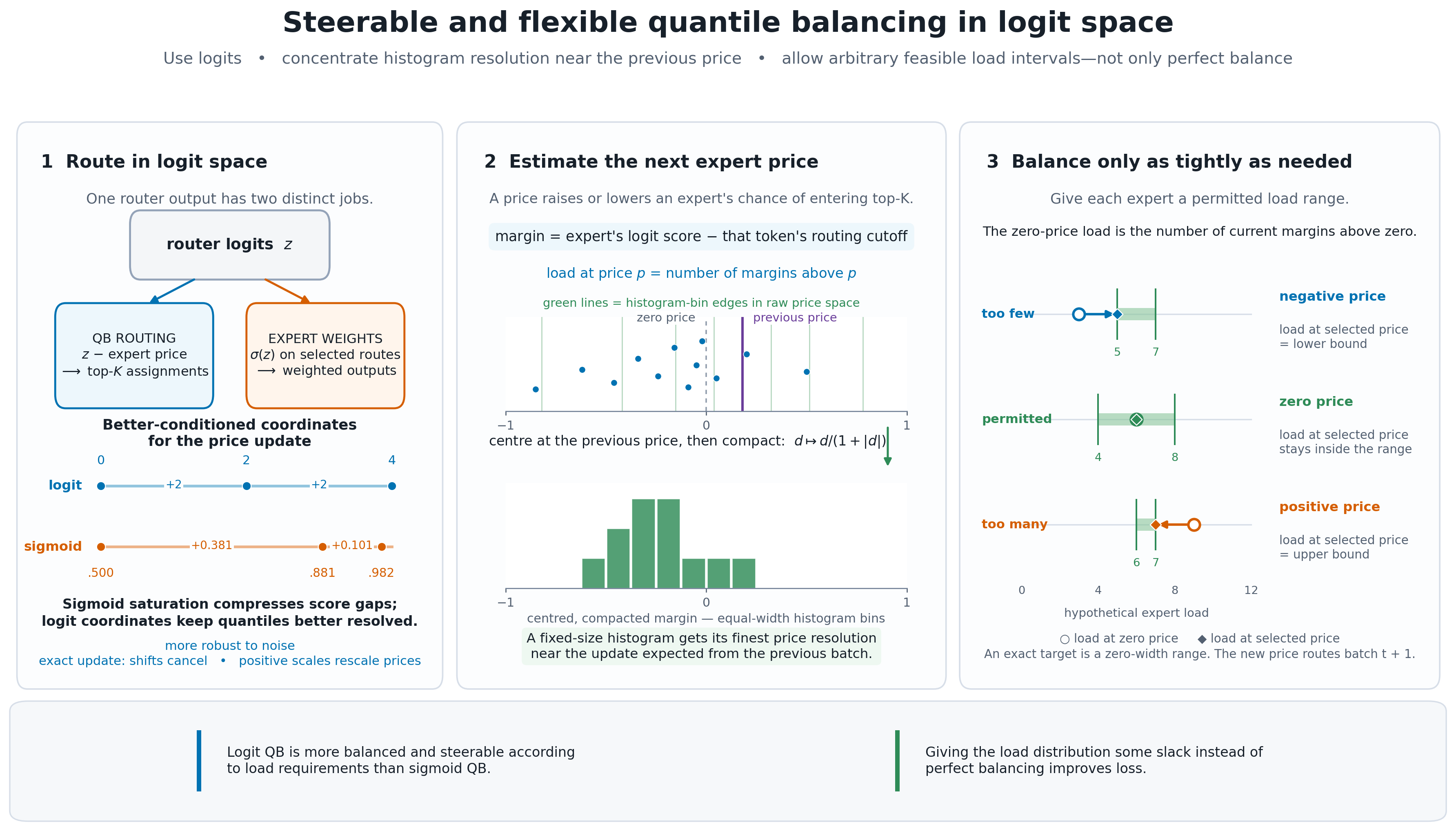
Considering this view, some desiderata of a good optimization algorithm, as well as other important aspects of the QB algorithm such as the score function and the histogram implementation, we come up with a generalization of the QB algorithm, which we then test across four different MoE sparsity levels.
We show two improvements - one for improving load balancing/steering of the load distribution, and another for improving loss by making load balancing strength configurable.
We find that using logits as scores for QB instead of sigmoid values (with different ways to compress these scores) makes quantile balancing much more accurate and steerable (as far as the requested loads are concerned), and that allowing for slack around the uniform load (flexibility around strength of balancing) improves loss, showing that perfect load balancing is not necessarily loss-optimal. The question of using it with a fixed exact non-uniform load distribution is still open. We also think about other possible algorithms under this view of load balancing, for the sake of completeness.
We also release code for reproducibility purposes.
Reading map
The following map/outline of the post is due to GPT 5.6 Sol.
If you are new to MoE load balancing, it is probably best to read the post in order. The first few sections explain why load balancing is needed, where the balance should hold, and why uniform expert loads are not necessarily optimal.
Readers already familiar with MoEs can skip the two collapsed sections Choosing the balancing granularity and A brief history of MoE load balancing (though they may connect with the rest of the post). The new material begins at Understanding and extending quantile balancing, and the empirical conclusions are in Improving quantile balancing: design and results.
If you mainly want implementation and training guidance, read Choosing the balancing granularity and then the score, experimental setup and results subsections under Improving quantile balancing: design and results. The mathematical section explains the theory, but is not required to follow the experiments.
If you mainly want the optimization argument, begin with Understanding and extending quantile balancing. It derives the assignment problem and its dual, connects some bias-update methods, generalizes the load constraints, and examines where the quantile update can fail.
Outline of the post
Introduction explains the two main reasons for balancing expert loads: preventing experts from being starved of training signal, and avoiding stragglers in expert-parallel systems. It also talks about logical imbalance across experts and physical imbalance across devices, the latter of which systems based on dynamic expert replication can partly address.
Choosing the balancing granularity talks about sequence-level, microbatch and global-batch balancing, and pruning for inference. It explains why finer-grained balance is more robust to distribution shift, gives a simple bound for mixtures of balanced subgroups explaining why, and discusses the corresponding tradeoff with expert specialization.
What should expert loads look like? asks whether uniform loading is actually the right objective. It discusses high- and low-frequency experts, shared experts and dense layers as ways to factor out common computation, routed experts as content-addressable capacity, and possible designs with several expert tiers, routers, sparsities or target ranges.
A brief history of MoE load balancing introduces auxiliary balancing losses, hash routing, reinforcement-learning approaches, global versus microbatch balancing, aux-loss-free bias controllers, SMEBU and quantile balancing. It places aux-loss-free and quantile updates within a common optimization problem that is discussed later.
Understanding and extending quantile balancing first gives an elementary two-quantile explanation: one quantile determines each token's routing threshold, and another adjusts each expert's price to obtain its desired load. It explains why the method uses the previous batch rather than repeatedly solving the current assignment.
The section then formulates top- routing as a degree-constrained bipartite assignment problem, establishes feasibility and integrality, and derives its dual. Per-token dual variables become routing thresholds, while per-expert variables become prices that discourage overloaded experts and encourage underloaded ones.
This dual view connects proportional and sign-based aux-loss-free updates to gradient descent, interprets quantile balancing as a delayed block-coordinate method, and generalizes it from exact uniform loads to per-expert load intervals and arbitrary exact targets. It also considers softer convex load penalties, explains why the quantile update has no general convergence guarantee, and gives an example of a suboptimal fixed point.
Improving quantile balancing: design and results looks at three choices that can be changed independently: the score used to value assignments, the desired load constraints, and the algorithm used to update expert prices.
Choosing the assignment score: sigmoid vs. logit argues that sigmoid saturation can make important score differences and quantiles difficult to resolve. It proposes using pre-sigmoid logits and compacting score margins relative to the previous expert price, which concentrates histogram resolution near the expected next update. It also discusses exact-quantile simulations, affine transformations, Moving Quantile Balancing and existing public implementations.
Experimental setup describes the four 285--293M-parameter MoE setups with varied active parameter counts, baseline and routing-parameter tuning, five-seed matched comparisons, and the metrics used to distinguish absolute imbalance from failure to follow the requested load profile.
Do logit scores improve balance and loss? finds that logits follow exact uniform targets more accurately in every matched comparison and generally follow slack or non-uniform targets more accurately as well. Exact-balance loss estimates all favor logits, although some of them are still inconclusive in a strict sense.
Relaxing exact load constraints motivates two alternatives to perfect uniform loading: allowing each expert a load interval, or prescribing an exact non-uniform load distribution. It argues that preventing expert starvation may matter more than tightly limiting heavily used experts, especially in very sparse MoEs.
Does load slack improve loss? reports lower mean validation loss for slack in all eight matched architecture/router comparisons. The selected bounds also suggest that keeping lower bounds relatively tight is more important than imposing equally tight upper bounds.
Do inverse-rank load targets help? finds no clear loss difference between the tested inverse-rank targets and exact uniform balancing. This suggests that freedom within a load range may be more useful than committing in advance to one particular unequal distribution, but could also improve with further tuning.
Alternatives to the quantile update asks whether more stable optimization methods could replace the delayed quantile step, and considers the computation, memory and communication costs that make otherwise attractive methods difficult to use during large-scale training.
We release code and configurations for this post at this link.
Introduction
When training MoEs, we want some amount of load balancing across experts, i.e., routed experts should activate at similar rates. There are at least two reasons for this - a training-related reason and a systems reason.
The training-related reason is, as discussed in e.g. OLMoE, Outrageously Large Neural Networks: The Sparsely-Gated Mixture-of-Experts Layer, and Expert Choice Routing, that not having load balancing tends to concentrate tokens on a small set of experts, and the starved experts remain under-trained, potentially leading to a feedback loop where better optimized experts get chosen more often.
The systems reason is that we want the model to be easy to serve (and train) - in an expert-parallel setup, where experts are sharded across GPUs/nodes, if there is a single replica of each expert, then the expert having to serve times the mean number of tokens will roughly take times more time than the average expert (as a first approximation). Having such stragglers is not optimal and from a systems perspective, having tokens spread out evenly across experts is desirable. One caveat here is that now there are already libraries for expert parallelism that dynamically replicate experts to have perfect physical load balancing across ranks (not logical load balancing across experts), such as MoonEP, and this straggler mechanism used to be more of an issue with DeepEP and such. Expert replication is still kind of messy, so some may still prefer load balancing for systems reasons too.
So we'll talk about how load balancing is done, what our desiderata might be, and two improvements on top of quantile balancing - one for improved balance/steerability, and one for flexibility (quantile balancing in itself does not have a way to control the amount of balancing).
Choosing the balancing granularity
Background: balancing granularity and distribution shift
Now that we understand that we need to balance token allocation across experts, let's think about the granularity we want the balance to hold on.
There are multiple possible granularities. From a serving perspective, one would want perfect load balance across the inference token distribution, and the ideal case is having such balance in every time interval, across all user queries.
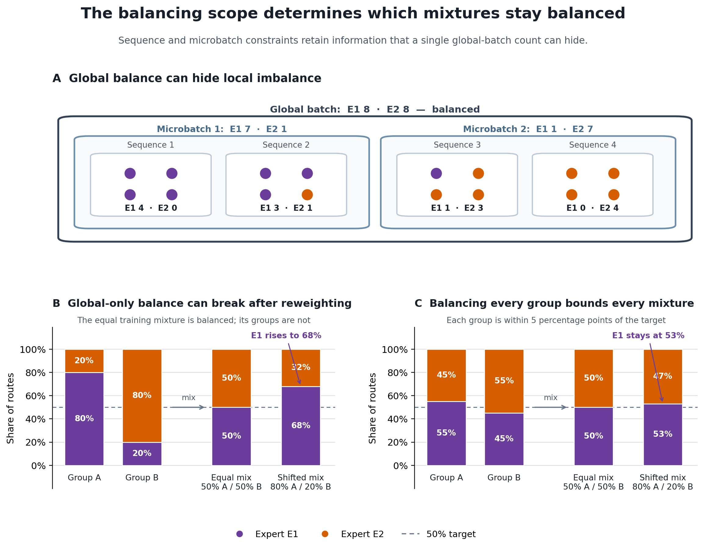
In training, load balancing is done either within the microbatch (or sequence-wise) or the whole global batch.
Note that a learned router would have at least some kind of specialization (not necessarily interpretable) as far as token/context distribution goes (otherwise we could allocate experts uniformly at random without quality loss). Intuitively, a router could learn to route to certain experts for certain kinds of documents/prompts (dictated by activation geometry). So under a distribution shift, we would see an increase in imbalance in a globally load balanced MoE. Typically, the finer the granularity, the lower one would expect the variance in the load to be, and a sequence or microbatch balanced MoE would be more robust to such distribution shifts - more specifically, let's say for each "subgroup" , we have a normalized load vector satisfying , then for any reweighting of these subgroups, the final load imbalance is . But this also trades off expert specialization and quality, so there may be an optimal non-zero extent of such balancing that can help the model in general.
As an aside, strong expert specialization can sometimes imply the existence of experts that are always active or are important in some other sense, so if a small set of experts covers the majority of experts used for a certain type of task, then things such as pruning or even loading these experts into faster memory (in e.g. heterogeneous memory setups such as local inference of large models with CPU offloading) can be considered. However, it does not seem likely that optimizing for this kind of human-interpretable expert specialization is optimal as far as loss/benchmark performance is concerned. One example is REAP, an expert-pruning method that seems to preserve performance on certain domains after pruning experts.
What should expert loads look like?
For now, we ignore the systems concerns (naively delegating all of them to something like MoonEP), as well as sequence-wise and microbatch load balancing, and think about how things should be, in an intuitive manner.
Let's fix a certain data distribution (say, the training distribution). If there is expert specialization, the load distributions over experts that we see in loss-wise optimal setups are not necessarily uniform. There might also be more than one of these optimum distributions, and load distribution is just a low dimensional observation of something much more complex. It would generally depend on the full training dynamics, through things such as the job of the rest of the architecture (e.g. whether or not we have shared experts or other similar mechanisms), what kinds of feedback loops exist/what instabilities we face during training (and which optima are actually reachable through training), how expert specialization happens (and in general, how the router is learned and its geometry).
One way to think about the optimal load distribution intuitively is by coarsely splitting experts into high and low frequency experts. For high-frequency experts, the routing for them can be approximated by them being always on (e.g., shared experts in a single layer or alternating dense/MoE FFN layers if we consider the whole network), and the rest of the experts are routed experts. Other aspects can also be important for routing - one can imagine a bias on top of a linear router or even a nonlinear router to improve routing quality as well as balance (and the ZAYA1-8B technical report shows that increasing the expressivity of routers empirically seems to help both quality as well as balance).
One might want to "factorize" out as much of this kind of behavior as possible in different ways (such as the shared experts in DeepSeekMoE or the alternating dense/MoE FFN layers in the MAI-Thinking-1 report), and keep the routed part of the MoE fairly balanced, because we want to both avoid routing collapse (because it leads to reduced expressivity) as well as not lose out on expressivity due to reduced expert specialization (as far as more obvious experts that can be shared/factored out in some other way are concerned). The former is the much bigger concern, because training stability in general governs many of the decisions made for large scale training runs.
Jianlin Su's blog series on MoE has yet another view of MoE as some kind of a "low-rank" approximation to the full dense MLP. In that sense, one can think of some frequent experts corresponding to certain "important" or "common" features (or something analogous to SVD modes), and the less frequent ones (or the ones to be balanced) as the more specific features that don't get activated all the time (but when they do, they end up being in the top few experts that matter as opposed to always having a tiny contribution).
Note that when we have shared experts, we can think of the model as a dense backbone plus some extra experts that need to be routed to - these are the extra parameters that potentially behave like a content-addressable memory (where the addressing is done by the router) and help reduce loss by storing "knowledge" without necessarily being active all of the time. The factorization might be important because if we do not do so, and have perfect load balancing, then if there is some shared work that is necessary to be done for every token, every chosen subset of experts has to do at least part of the work that this shared expert would have done, reducing the available capacity for expert specialization. Tuning the number of shared experts can help.
It is still unclear whether this 2-way factorization is optimal or not - it might very well be possible that the optimal way would have more tiers to such routing while still controlling how the router works (we can have multiple routers, each balanced separately, with different expert subsets with different sparsities, a special case being shared experts corresponding to the trivial router plus the rest of the experts with another router, or a load balancing setup that has different load targets/target ranges for different experts, all balanced at the same time, or even learned-routing-free methods such as hash routing for some subsets).
A brief history of MoE load balancing
Background: representative load-balancing methods
The traditional way to achieve load balancing has been adding an auxiliary loss term, called a load balancing loss, which is a loss that is minimized when we have perfect load balancing, as in the original sparsely-gated MoE and the Switch Transformer. The tradeoff between expert specialization/model quality and perfect load balancing is decided by the coefficient of this aux loss term as compared to the usual modeling loss term.
An alternative is hash routing - instead of a learned router, it hashes some kind of token (or n-gram) information and maps these hashes to the experts in some way (optionally in a Zipf-aware manner for balance). This works surprisingly well, though learned routers are generally supposed to be better.
Another historical method was to treat routing as an RL problem (a natural choice considering routing is discontinuous), as in Conditional Computation in Neural Networks for Faster Models, but it turned out that this was overkill.
In practice, people now use a global load balancing loss and it tends to work quite well (people typically used microbatch load balancing earlier) - Demons in the Detail compares global-batch and microbatch load balancing and also discusses the effect on specialization.
DeepSeek introduced aux-loss-free load balancing, which does not require an auxiliary global load balancing loss (but DeepSeek still used one for sequence-level load balancing to avoid extreme load imbalance within sequences). The idea is to decouple expert selection from expert weighting to a certain extent. Traditionally, the same gate value is used to weight experts (alongside normalization) and to choose experts for a given token. Let's say is token 's score for expert . Then instead of , selection in this method uses for top-K choices, and is not optimized using typical gradient descent. Rather, it is treated as a per-expert controller, and the updates to it are done in a direction that restores the balance for a given expert (e.g., if the load is higher than desired, is reduced by a constant, and vice versa). Other variations also exist, such as SMEBU which improves upon the brittle sign-like updates and smooths them using momentum as well as a smoother replacement of . In general, routing gradients do not seem very well understood as far as load balancing is concerned, so having this optimization be a separate problem makes things somewhat cleaner.
Quantile balancing uses a similar controller idea, and, intuitively speaking, tries to solve for the correct biases directly (approximately). It formulates it as an optimization problem, and while aux-loss-free optimization can be thought of as some kind of dual descent for that problem, quantile balancing is a way to do something like a block coordinate descent to solve the same problem, but in an amortized (and stochastic) manner over multiple training steps. We will explain this in the next section.
Also note that there are many other algorithms that we will not cover, in order to avoid overwhelming the reader. The algorithms mentioned above are only representative of the ones that have been prominently used in large training runs.
Understanding and extending quantile balancing
There are two ways to understand quantile balancing. The first is an ad hoc way and is a bit easier to think about in an elementary manner, and the second one is a more theoretically grounded way and also helps us generalize quantile balancing (which we will do in this section).
To gain some intuition, let's first look at expert-choice routing (what we had been talking about so far was token-choice routing). In this type of routing, experts choose tokens based on their allocated capacity. In this setting, we can have perfect load balancing, but at the cost of causal leakage - a routing decision made for an earlier token based on a later token can act as a side channel for information, and for large models it can let the model use this to predict the next token much better, while not being compatible with (and worsening the performance at) inference. It also causes information leakage across different sequences in a batch. Note that in the case of token-choice routing, dropping tokens itself (when experts have hard capacity constraints) can lead to causal leakage too, depending on implementation (in general, strictly causal decisions on dropping tokens can lead to a strong positional bias in which tokens are dropped or lead to wastage of capacity if some kind of budgeting is done, so load balancing is important here too).
Still, we would like something that has as good of a balance as possible. Assuming that the token distribution doesn't change much from batch to batch, it might be fine if we accept a delay of a single step when optimizing for perfect load balancing for a top- token-choice MoE.
Let's say we have the scores for an expert for a token (these can be completely unrelated to the gate values, but in the standard quantile balancing setup, they are taken to be the same). Let's interpret the biases as "costs" (and use this time, so that demand for an expert increases its cost).
We now want to update the biases from to so that after the update, we have reasonable balance.
Now, consider a single token. To be in the top experts (out of ) for a token, a given biased score needs to beat the -th largest value of all the expert biased scores (taken over ). This gives us a threshold for each token as a quantile of the biased-score distribution of experts for that token. Now, suppose is fixed. In the spirit of alternating optimization algorithms such as EM, let's try to "solve" for assuming is constant (that is, the thresholds are frozen). For a given expert , we want tokens (out of a total of ) to have their cutoff be satisfied by this expert. As earlier, this happens if , or equivalently , for tokens out of a total of tokens. Thus, the new bias is again a quantile but this time of a distribution of biased scores over tokens for that expert.
In most cases, intuitively, this iteration, if carried out on the old batch, should get sufficiently close to the bias that solves the problem optimally. However, this needs us to compute statistics over a batch repeatedly and has non-trivial communication overhead, so the quantile balancing method does only one step (instead of iterating to convergence) and tries to amortize across steps in a similar vein to minibatch stochastic optimization methods.
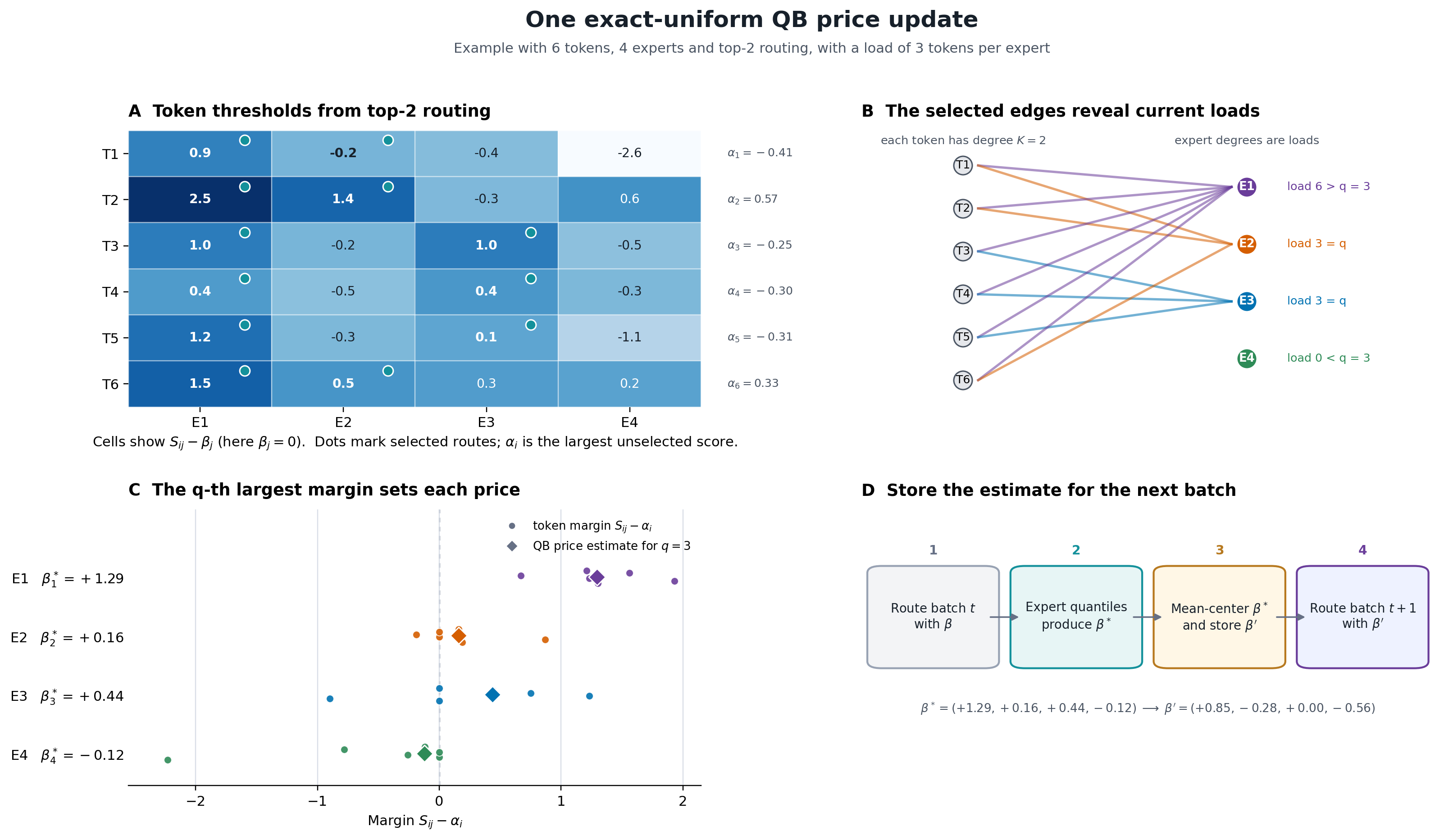
Let's now look at it from a slightly different perspective. The following approach, for the special case of perfect balancing, is mostly covered in the Kimi K3 report, but we will generalize it below.
Matching tokens to experts is a bipartite matching problem but with more general degree constraints instead of the usual unit degree constraints. To see why, let's draw a bipartite graph, with tokens on the left and experts on the right. Each expert has a specific number of tokens it is assigned, which will be its degree in the matching, and each token has experts that it will be assigned to (i.e., their degrees must be ). The Gale-Ryser theorem gives us a condition for when a balanced matching exists and we'd need to verify it to check feasibility. It states that non-increasing non-negative integer sequences and are the two degree sequences of a simple bipartite graph if and only if their sums agree and, for every ,
When we require perfect balance (i.e., all experts have the same degree and all tokens have the same degree), the condition in the theorem is trivially true, and a balanced matching is guaranteed. Even when we have arbitrary degree constraints on experts while all tokens must have the same degree , it is fairly mechanical to verify that the Gale-Ryser condition is satisfied as long as the expert degrees sum to and the degrees are bounded by their trivial bounds.
In fact, we can make this a bit more general. Let's say that token can be assigned to between and experts (this specific generalization is not useful for usual top- MoEs, but we keep this regardless for generality), and expert can be assigned to between and tokens (this specific generalization is important if we want to have slack in our expert loads or arbitrary exact loads and so on), and assume that these thresholds are such that there exists a solution to this assignment problem. (Also, we assume that these bounds are integers and are bounded by the natural bounds one would have for degrees). The case where and corresponds to the situation above. The analysis for the special case of perfect balancing (plus ) is a bit easier, but we will deliberately use the more general case to be able to generalize quantile balancing further.
Now we need to choose one among these balanced matchings. To do so, we need to define the quality of a matching. We define it as
where is the score given by token to expert , and is if token is routed to expert and otherwise. Note that is not necessarily related to the gating score in this formulation, but it is taken to be equal to the gating score in quantile balancing, intuitively because a better expert should have a higher score. Later, we will see how taking to be the post-sigmoid gate and the pre-sigmoid gate logit makes things different, so it is worth thinking about as a value we use for defining an objective function, separately from its utility as a gating function (which is also helpful for gradient flow through the router).
Note that is a discrete binary variable here. Let's for the moment relax its domain to . For the moment, for perfect balancing, assume that is an integer.
We want to show that all the vertices of the polyhedron corresponding to the equivalent linear programming problem are integral, so that for each linear "quality" function, the optimum value of the function is achieved at an integral point (as opposed to only at points where is fractional for some ). This follows because the optimum of any linear function is achieved at an extreme point of the polyhedron.
There are two ways to approach this.
Proof using total unimodularity.
The first, a bit mechanical, way is to try and show total unimodularity of the matrix that defines the polyhedron, i.e., any square submatrix has determinant or . Let . Then if is the vector of upper bounds and is the vector of lower bounds, then defines the polyhedron, where is formed by stacking and is formed by stacking respectively. To show that is totally unimodular, we only need to show that is totally unimodular (easy to reduce). For this we consider expanding a submatrix along a column - any column has at most two -s. If there is a column with at most one of those, expanding along the column lets us induct downwards. Otherwise every column has exactly two -s - in which case, it corresponds to an edge, and the two vertices correspond to an expert and a token. Now partition the rows (corresponding to a vertex) into experts and tokens, and sum them - both sets of them sum to the all-ones vector, so the rows of are dependent, in which case its determinant is , and we are done.More intuitive proof using flows.
The second way is a bit more intuitive, and that is to treat this as a flow problem. For a bipartite graph (with vertices on the left being , on the right being , and edges being ), add a source vertex and a sink vertex , and construct the following edges with the mentioned flow constraints: with , with , with iff is an edge, with . A feasible assignment gives rise to a circulation on this flow graph uniquely. Now consider a fractional . First note that there can't be exactly one fractional directed edge incident to any vertex (due to flow balance conditions) in this flow graph, so if we consider the vertices that are incident to any fractional edge, the minimum undirected degree in that graph is , so it must contain an undirected cycle. Since all the edges in this undirected cycle are fractional, we can choose an appropriate such that we can "send" a circulation of along this undirected cycle (with appropriate edge signs) while the flow constraints are still satisfied. But in that case, is a midpoint of two other feasible points in the polyhedron, which means it is not an extreme point.So, we have shown that it does not matter if we relax our integer programming problem (corresponding to assigning experts to tokens) to a linear programming problem. This means that we can use standard ideas from optimization.
Let's write the original linear programming problem for a top- MoE again: subject to , , . Here we enforced each token to use exactly experts to reflect that we use top- MoEs as well as to simplify the analysis.
We now think about the Lagrangian. To do this, introduce a variable for each constraint of the form , for , and for .
Consider the sum
Define . Note that under the constraints on and , we have, for any feasible , that , so is an upper bound on the value of any feasible matching. So we can minimize this over the multipliers and to get the best possible upper bound on the value of any feasible matching. Strong duality says that, since this is a feasible linear program, this bound is actually tight. That is,
Now, let's rearrange and perform the inner maximization to get the maximum value as:
which equals (by choosing appropriately)
Let's define as the signed "price" (we explain this terminology later) of the expert (for now, this is just how and appear in the non-linear part of the objective) - then the summand on the rightmost end is minimized when and . Substituting and defining for and otherwise, we get
As an aside, let's see what is really about. In the case where , becomes a linear function. Otherwise, it has an interesting interpretation - if we instead parameterize the slack interval as being centered and within of it, then is . This is equivalent to adding an L1 penalty on on top of the original problem, leading to some bias towards sparsity.
Let's first try to eliminate . For fixed , it is a convex function in each separately, with the (global and local) optimum being when the slope (subgradient) is , i.e., is non-negative (define slope at arbitrarily) at values of , i.e., is anywhere between the -th and -th highest values in (so it corresponds to setting the corresponding to the top to and the rest to , modulo ties). So the minimization objective becomes .
Before deriving quantile balancing here, we pause to see what happens if we throw gradient descent at this problem, as noted in the Kimi K3 paper for exact balance without slack. In the case of exact balance without slack (i.e., is linear and equals ), away from ties in routing, the gradient becomes exactly the negative of the imbalance, and the gradient descent step increases if the expert is overloaded, and reduces if it is starved. SignSGD instead of gradient descent gives DeepSeek's aux-loss-free load balancing, and e.g., SMEBU from Arcee Trinity Large is a soft version of it, somewhat reminiscent of an Adam-atan2 + LaProp style version of the algorithm.
However, if we had some slack, the gradient step would look like this: if (i.e., the cost of choosing an expert is positive), then we look at the upper bound - if it is violated, then we increase by a value proportional to the violation, and if it is not, we reduce it by the same amount (note that we are being deliberately conservative in updating so that only the bare minimum for keeping the load within bounds is done). Something analogous happens for the lower bound. However, if , then we update only if there is any violation, and update it in the correct direction; if there is no violation then remains . Doing a SignSGD step here like in the aux-loss-free load balancing family of algorithms would work too. Note how we get an analogue for a with-slack version of load balancing almost immediately.
One may ask, why not solve the optimization problem optimally in the first place, instead of using gradient descent? After all, gradient descent or SignSGD have the issue that the step sizes for are not sensitive to the score density near the margins (and an update size that does not take this into account can lead to either a drastic change or a negligible change in load) - standard Newton-ish methods could be worth trying too, though second-order estimation could be an issue (and besides, this is a pretty discrete problem, so it would need some kind of continuous approximation).
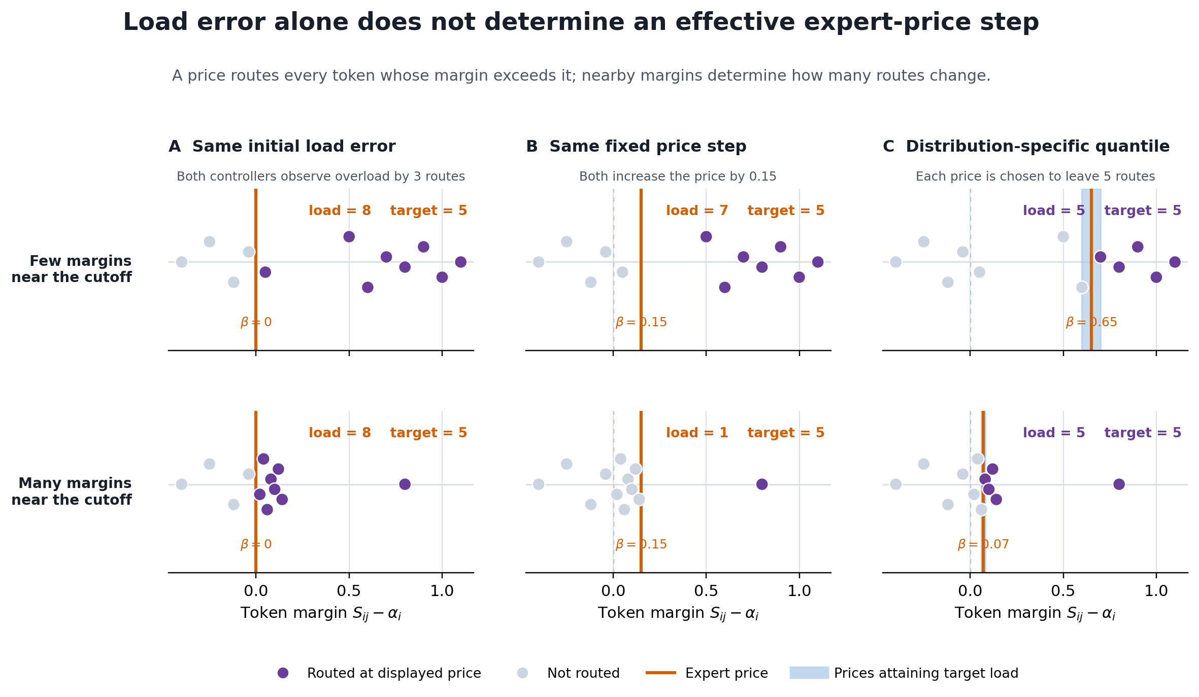
The naive way is to try and solve by noting that this is a convex optimization problem. However, this does not have a closed form, and typical convex optimization algorithms are iterative in nature. In particular, if they require computing the objective function or a subgradient many times, it could get expensive quite quickly. Also, if the batch is small enough, fitting to the current batch perfectly is likely to be suboptimal for the next batch (and would necessitate some kind of proximal penalty for things to be stable across steps). So we would like to do a single iteration (or a few iterations tops) of any such algorithm, taking inspiration from stochastic minibatch optimization algorithms. Note that approaches such as bundle/ADMM/primal-dual algorithms/LP solvers/Sinkhorn-style approaches can be quite expensive (computationally or memory/communications-wise), so we don't pursue them here.
Since this form of the problem doesn't look as tractable, let's go back to
We can try and solve this problem using blockwise coordinate descent (i.e., alternating between optimizing over and while keeping the other fixed), and it has a simple and fast closed form iteration. For the special case of perfect balance, we see that this recovers our old balancing - optimizing over while keeping fixed gives the top-K sum as earlier, and the is the threshold we need to cross to get into the top of the biased scores (consider what happens when we pair up each copy of with each active expert). The same argument when we keep fixed gives us the equivalence for the update in our old analysis and this setup.
Let's reason about it again in the most general case, to generalize quantile balancing. When optimizing for , nothing changes because is separate, and it leads to the same definition that leads to them being the top- cutoffs for a given token. When optimizing for , things change a bit.
Note that is a privileged value in the general case (unlike the standard quantile balancing setup, where we can shift all the by the same constant and it would not affect the result) - this is because , and at most one of the and is non-zero as we saw earlier - positive corresponds to a positive , which is used to penalize an expert that would be over-selected if no penalty was applied, and a negative encourages an otherwise under-selected expert to be selected. If both are , it means the expert is already fine and needs no help. In some way, since is the threshold vector for each token, and it is decided by the value of , can be thought of as a price that one has to pay for an expert (while gaining from being allotted that expert) and this is decided by the demand/supply situation due to the forces wanting to have expert balance.
Keeping fixed, the problem for a given expert becomes, defining as the margins for token for expert , . This is a convex problem, and its local minimizers are also its global minimizers, and have zero in the subgradient. In what follows, we will ignore ties to make our life easier. Let be the number of tokens whose current margins for this expert exceed - this is a non-increasing function of . Then for , the derivative of the objective is , and for , the derivative is .
Now we derive the update - if we have , we can just set . If , since is non-increasing, the minimizer satisfies - in which case we find such that . Similarly, if , we find such that . This is the same as finding the (usually non-unique) quantiles corresponding to either or , and is a natural generalization of the standard quantile balancing update from Kimi K3 (modulo how the exact inverse-quantile value is chosen - this is non-unique due to gaps between token margins).
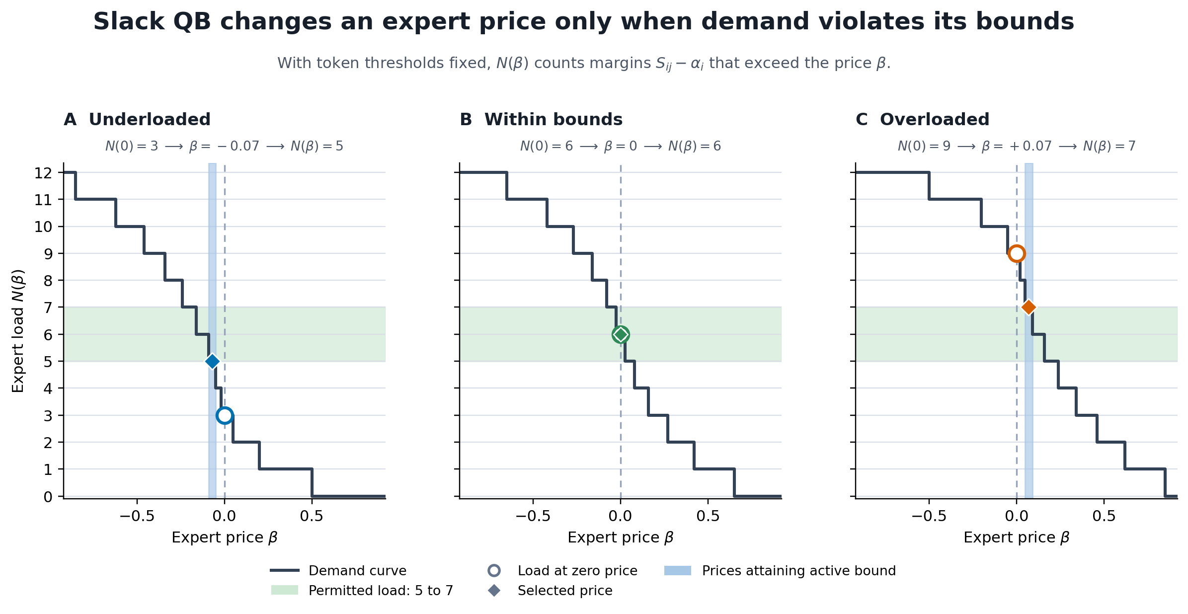
An important detail to be kept in mind is that since this is a non-smooth problem that is also not "separable" into the blocks of and that we perform block-coordinate descent on, this algorithm does not necessarily converge, either for standard quantile balancing or our version. There may be non-benign oscillations that don't converge to the optimum (there do not seem to be any convergence guarantees from theory), but also, the convention we use can also get stuck at a non-optimal point (for the latter, consider , , - starting at gives and as a fixed point, with the dual objective , whereas the optimal assignment is , , whose score is , so the solution found was suboptimal).
One way to reduce noisy assignments could be to check at the old first, to avoid jitter from our quantile/0 assignments (or even overfitting to the new batch), but we don't pursue this. Another way is adding a penalty such as for or or something similar - this still keeps the problem convex as well as solvable in the same step (potentially needing a binary search), but again has the issue of not being equivalent across experts - ideally such a penalty has a geometry that respects the relevant score density, which we will not pursue further due to its complexity.
Another aspect to think about is that hard constraints might not necessarily be good, and that the effective might be better off being smoother, and it is possible that in the current formulation for infinitely large batches, expert load gets stuck at the boundaries for many experts. One way of thinking about this could be the following: as we already noted, is a sum of a linear term and an L1 penalty - this L1 penalty controls how much load balance matters for us (and the shape of is a plausible way of controlling what load profiles matter for us). To control this "profile importance", we might want some kind of principled way of thinking about 's shape - it should presumably be convex (to keep the problem convex). As it turns out, there indeed is a way of doing so, and that way derives as a convex conjugate of a penalty being subtracted. Instead of hard constraints, we add a penalty term on the per-expert load in the primal objective that we want to maximize, say , where is the load on expert , and we also keep the primal top- constraint (i.e., becomes with , call this constrained set ) instead of dualizing it. Note that integrality of the optimum doesn't carry over for general , but we will still think about this nevertheless. If is the convex conjugate of , then . Plugging this in, we get . If this satisfies the finite dimensional Fenchel-Rockafellar conditions, then we can swap the and , to get , which shows that corresponds to the role of a convex conjugate of the negative of the penalty, and indeed, the convex conjugate of is the indicator function of the interval ( outside the interval, inside the interval). Of course, if is not piecewise linear, one would in general need a binary search (or similar) to find the zero subgradient points.
It is also possible that noise softens the boundaries more than the hard constraints tell us, because we have to satisfy the "oracle" balance plus the noise, instead of just the oracle balance. Solving the problem exactly is also likely not ideal, because as we mentioned earlier, the optimal -s can be very different between batches (and also be overfitted) unless we have some kind of regularization/damping towards the previous .
We tried two special cases of this generalization and compared it to the usual perfect-balance QB setup. In the slack setup, we use . The other setup has no slack but a different exact load assignment for each expert, proportional to for the -th expert, for a specified value of . The results are discussed later.
Improving quantile balancing: design and results
Let's first list down some considerations one may have for a method of solving the load balancing problem, and think about them in relation to quantile balancing.
For an online/stochastic optimization algorithm, there are some things we care about, such as robustness to noise, convergence speed, proximity to the previous iterate/staying within a trust region, and flexibility/generality in a meaningful way. We also care about the implementation being reasonably fast (either exactly or while being a reasonable approximation).
Let's come back to quantile balancing. Specific to quantile balancing, there are a few things: the objective function (linear sum of scores), the constraints (exact balancing), and the actual optimization algorithm (histogram-based block coordinate descent like stochastic algorithm amortized over the run).
Choosing the assignment score: sigmoid vs. logit
As far as the objective function goes, it is unclear what the scores for a given token-expert assignment should be. Standard quantile balancing (as done in Kimi K3 and the Jianlin Su blog posts) uses as the gate value. A motivation for the score being monotonic in the value of the gate is that the gate affects the expert's magnitude of contribution, so it is in some sense an importance score. However, this does not tell us that it must be the gate value itself - why not a higher power of the gate (such as its square), or the gate's pre-sigmoid logit? One way to interpret the objective function is how it scores things - for a sigmoid gate, it may not differentiate much between a gate value of and , but the pre-sigmoid logit score would (which could be either beneficial or not). In the end, the ideal case is that we have good (or at least steerable) load balance while also having better loss.
Note that different score functions will generally lead to different optimal assignments. In the case where the optimal choice of score function is not clear from a loss or training dynamics perspective, we may want to turn to other desiderata, as long as it does not adversely affect the loss and other things we care about. So in some sense, we have some freedom of choosing - for our experiments we choose the pre-sigmoid logit as one choice. On a skim, it might seem like a natural choice since it is more likely to behave like a typical pre-activation of a neural network (which in literature is typically assumed to be Gaussian-like or just constant std with both positive and negative values and doesn't necessarily saturate) than the sigmoid. But there are other more important reasons behind this choice, which are: compatibility with implementation, robustness to noise, and equivariance under linear transforms, and we discuss these below.
Consider the implementation for quantile balancing - it requires us to compute quantiles of a quantity over all tokens, for each expert separately (the other quantile computation is fairly simple to do locally). However, doing this exactly has a non-trivial communication overhead, especially in large scale training. The Kimi K3 paper's solution to this is to use a histogram - since the scores are all sigmoids (and hence bounded), one can just compress things into a to range. The paper claims that the error in is governed by the bin sizing. However, this is not the full story - consider a router with a low logit temperature (or low entropy in some sense, for a single token). Scores then concentrate around 0 or 1. Similarly (but a bit less crucially), when the router has a high logit temperature, the bounds on sigmoid are not tight (the actual part of the support being used is small), and many bins are wasted. If you recall the discussion on Newton-ish methods from the previous section, for good load balancing, it is not only these bin sizes that matter, and we need to also care about how the biased scores are packed within bins, for good quantile estimation as far as the resulting load error is concerned (e.g., in an extreme case, a bin can have the entire distribution and not provide good enough resolution even after interpolation, which assumes a uniform distribution inside the bin). So for a loose analogy, this is like using Newton's method or some other second order algorithm for an ill-conditioned problem under low precision.
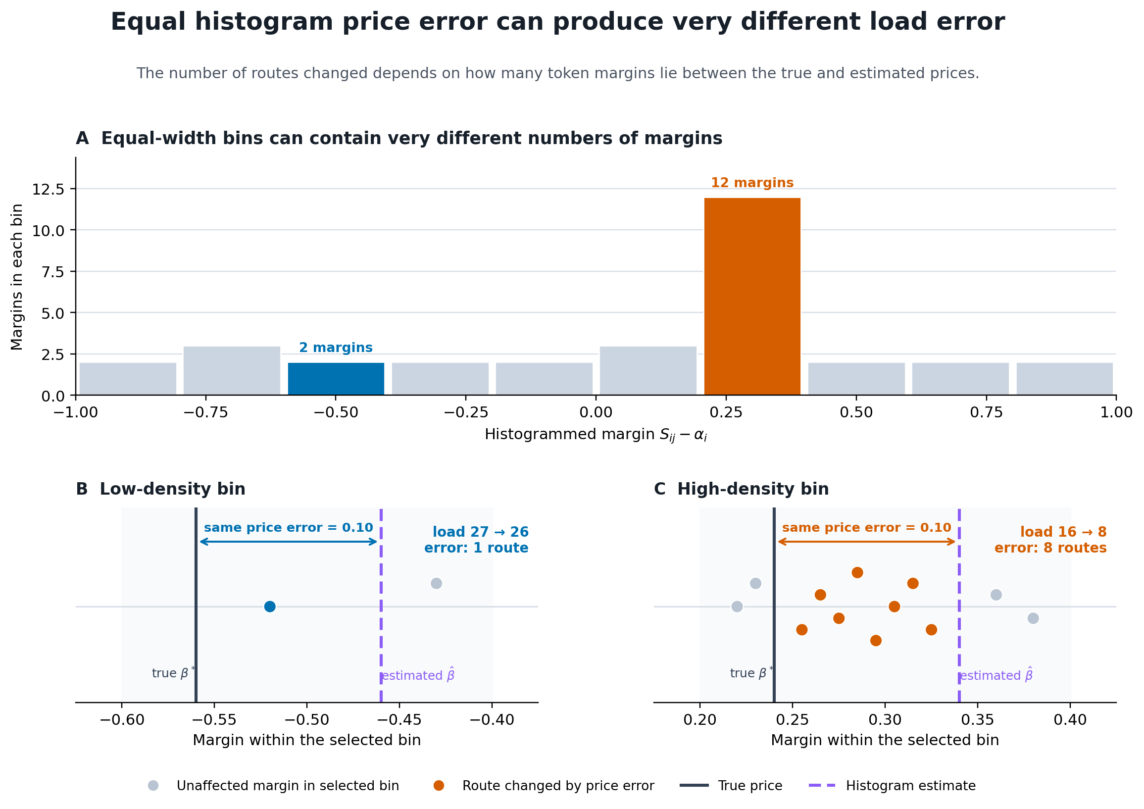
For a given expert , we want to compute a quantile of over all tokens . When is a pre-sigmoid logit, one issue we face while trying to apply compression is that it is not bounded naturally like sigmoid is. So we need to compress the quantiles from to some bounded interval (say ), while also preserving the resolution at the tails more than e.g. sigmoid, for extreme sparsity. One way of doing so is to use the map (we name this "compact"), and indeed we use this for most of our experiments. However, there is a better way. For a sensible optimization algorithm, one would expect that and the distributions of do not change too much between consecutive batches. In that case, the relevant quantile of would roughly be zero. So if we compress these values instead of , with an compression function which has a good resolution in where is the typical change in between consecutive steps, we have already solved this problem to some extent (it is likely possible to improve it by estimating , but we just use the same compression function after this shift; we call this method "relative-compact"). We notice the most stark benefits of this in settings where the desired expert loads are highly non-uniform.
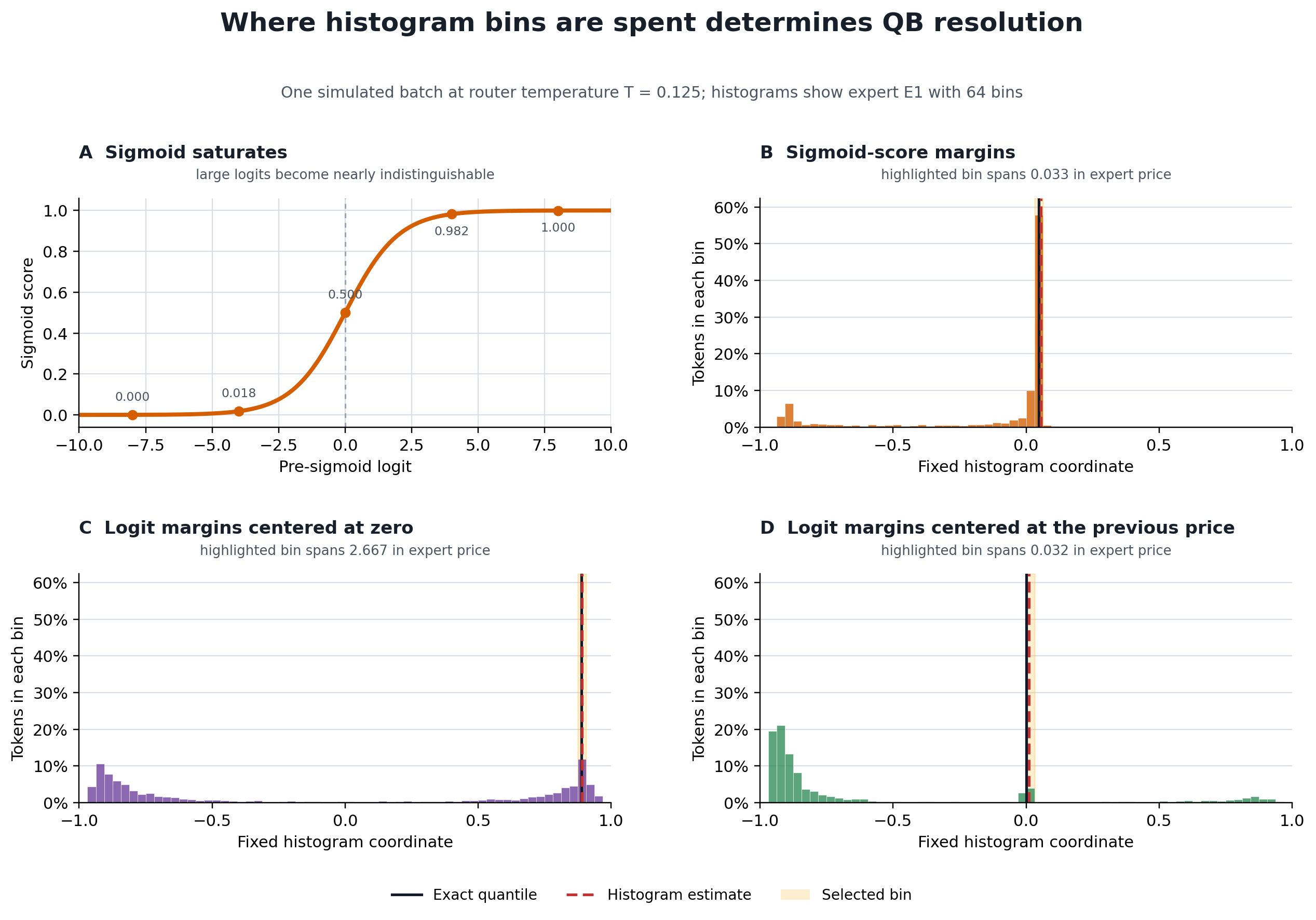
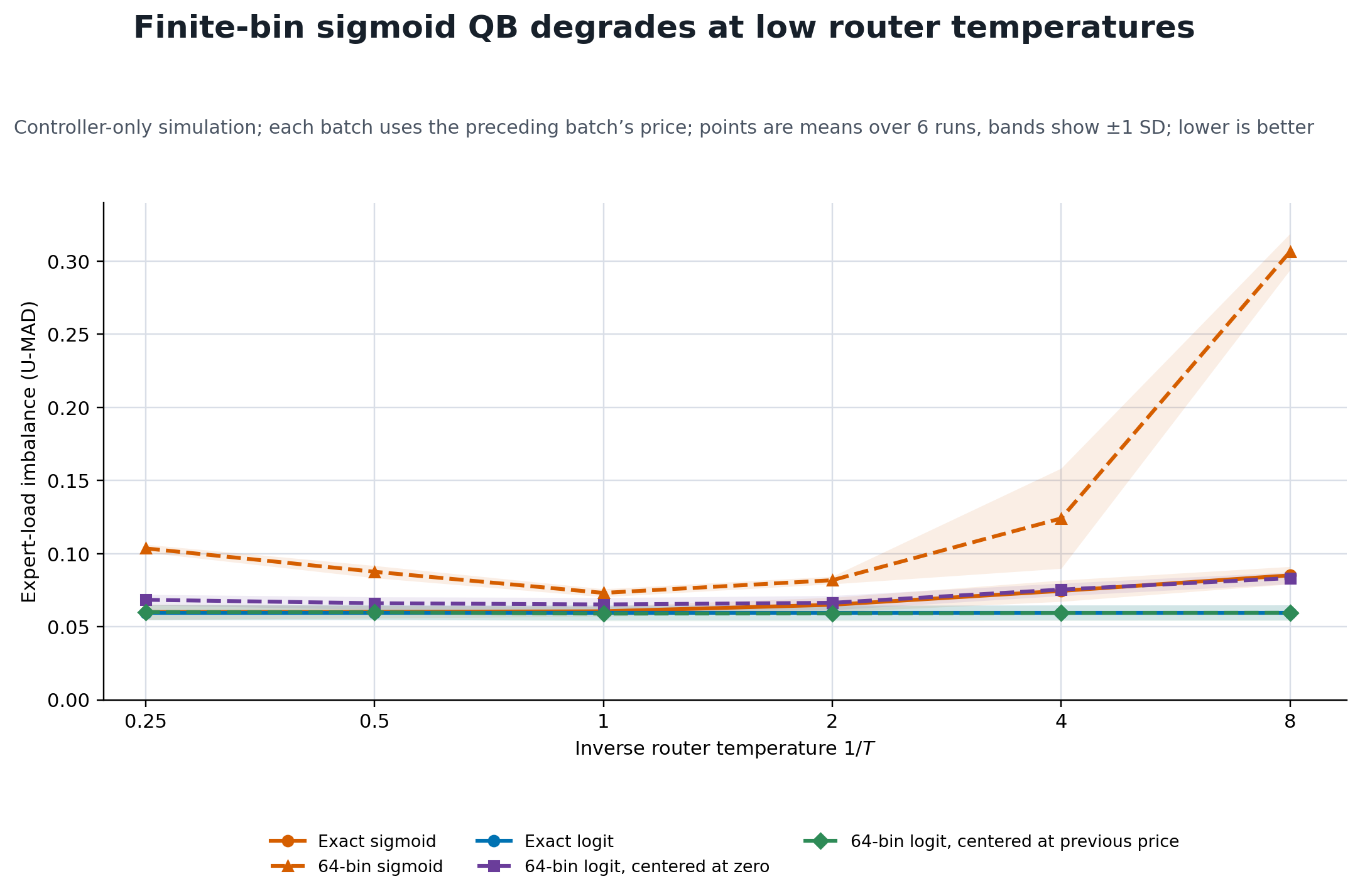
So the above deals with histogram resolution as a potential issue, which can also be verified using numerical simulations. But what happens if instead of using a histogram, we just used the entire distribution, with the caveat that we still have minibatch noise (so perhaps it does not matter as much at large pretraining batch sizes)? Does sigmoid still fare poorly? The answer seems to be yes, at least a bit worse, if one checks numerical simulations for instance. A somewhat nice theoretical aside is that when we transform the logits by a positive scaling and a translation, and both translate by the same amount, so the things we need to take the quantile of scale by the same amount. Under the exact setting (no histogram), this changes the "conditioning" everywhere uniformly, unlike in the sigmoid case, where things can start to concentrate in different places.
As an aside, note that, as mentioned earlier, we don't necessarily have to limit ourselves to global load balancing, and that it might be good to have some "local" load balancing such as across sequences or microbatches. Moving Quantile Balancing (MQB) by Jianlin Su is one way to do so for sequence-level load balancing. It maintains a histogram (using an EMA) that is causal and its strength is controllable by a multiplier . We don't focus on it here, however.
When I looked at the public implementations of quantile balancing after running the experiments below, the situation was a bit varied. The initial Megatron implementation uses QB with raw router logits, as we propose, but it also does not use a histogram (and instead uses a crude approximation by averaging per-microbatch quantiles). It cites Marin which implemented quantile balancing, and one of their agent-generated reports says that using the sigmoid gate instead of pre-sigmoid logits was catastrophically worse (in their setup), and compression also made things much worse for them. Separately, NVIDIA's Kimi K3 support tracker links to a global-batch histogram implementation PR which tries to match K3 by applying QB to raw sigmoid scores and using histograms too.
Now let's look at how sigmoid vs logit fare, at four different sparsity scales. The hypothesis here is that logit would be better than sigmoid as far as balance is concerned, with potential benefits in loss, but not guaranteed.
Experimental setup
Architecture, tuning, and metrics
We use a fairly standard transformer backbone which can be seen, alongside optimization details, in code. For the MoE layer, we use sigmoid routing, one shared expert, Kimi K3 style RMSNorm after combining routed experts. Model sizes are (total/active, including embeddings/lm head): 293.3M/15.5M, 293.3M/26.1M, 285.5M/29.6M and 285.5M/38.0M respectively. So experiments are quite small scale, but we may expect many of our proposed improvements to hold at scale, and at least motivate larger-scale testing.
The four sparsity setups are D384-R2 ( (shared + routed / total)), D384-R8 (), D512-R2 () and D512-R4 (). We first tuned strong standard QB baselines (for optimal loss) for all eight sparsity/router combinations with thousands of HEBO trials (HEBO was run on each setup independently) as well as sharing top configurations across stages (to reduce issues related to one router family or the other being harder to tune), and different seeds across search trials to avoid bias. After selecting those baselines, we froze all other hyperparameters and tuned only the routing-specific slack bounds or inverse-rank offset (this makes the results for our new changes pessimistic, and retuning can likely help increase the gains we see, but we didn't pursue this further). In the end, we ran the best candidates with the same 5 (held-out) seeds, and we report the means over those seeds. Paired comparisons are done using the same seeds, and we also compute the 95% paired intervals. For potential improvements (loss-wise or balance-wise) to quantile balancing, we only test the hypotheses we mention below instead of iterating.
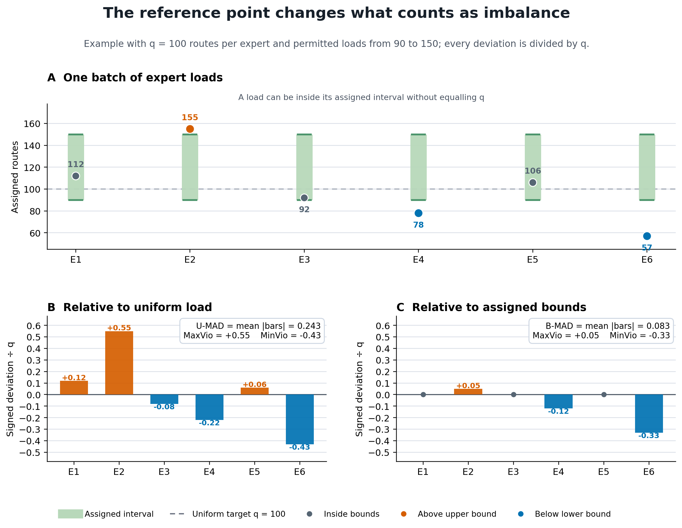
For balance, we look at two values, one for absolute balance and the other for "steerability". Let U-MAD be the mean absolute deviation from uniform perfect load, divided by that perfect load. Let B-MAD be the mean absolute distance outside the desired per-expert bounds, divided by the perfect load again. For exact uniform balance, they coincide, but for slack and inverse profiles, U-MAD tells us about imperfect load balance and B-MAD tells us how accurately QB follows the desired interval/target. We also report the corresponding signed extreme violations. MaxVio is the largest overload and MinVio the largest underload, and there are two variants: for the uniform-reference variants, they are the maximum and minimum of ; for the bound-reference variants, loads inside their assigned interval have zero violation and loads outside it retain the sign of their distance from the nearest bound, again divided by . We report both the mean across MoE layers and the worst layer. Each table entry is a five-seed mean computed after the layer aggregation within each run. The routing statistics are for the final training batch under the previous bias, while val loss is computed using the bias updated from that batch. Noise in val loss was typically around .
Do logit scores improve balance and loss?
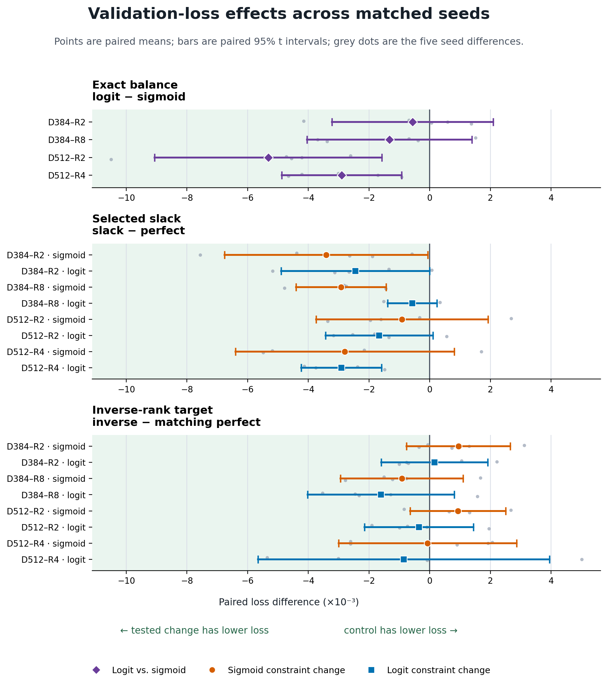
We compare the sigmoid and logit versions of QB below. The loss difference is logit minus sigmoid (so negative loss difference means logit is better). "Perfect compact" refers to perfect balance using for logit and the standard setup for sigmoid, "perfect relative" refers to centering using the old bias before using for logit and the standard setup for sigmoid, "slack" refers to relaxed load bounds, "inverse" refers to the setting with the expert loads, and is the number of routed experts.
Full sigmoid/logit comparison table
In the last four columns, U means the uniform perfect-load reference, B means the assigned-bound reference, and S/L means sigmoid/logit. Each entry is a signed pair. The U and B columns coincide for exact-uniform settings by definition.
| Architecture | Pair | Parameters (sigmoid / logit) | Val loss (sigmoid / logit) | Paired loss difference [95% interval] | U-MAD (sigmoid / logit) | B-MAD (sigmoid / logit) | Mean U Max/Min (S/L) | Worst U Max/Min (S/L) | Mean B Max/Min (S/L) | Worst B Max/Min (S/L) |
|---|---|---|---|---|---|---|---|---|---|---|
| D384-R2 | perfect compact | -- | 2.901449 / 2.900888 | -0.000560 [-0.003219, +0.002099] | 0.0782 / 0.0532 | 0.0782 / 0.0532 | S (+0.4281, -0.2369) / L (+0.1937, -0.2301) | S (+0.6380, -0.4342) / L (+0.3201, -0.4462) | S (+0.4281, -0.2369) / L (+0.1937, -0.2301) | S (+0.6380, -0.4342) / L (+0.3201, -0.4462) |
| D384-R2 | perfect relative | -- | 2.901449 / 2.900683 | -0.000766 [-0.004327, +0.002796] | 0.0782 / 0.0537 | 0.0782 / 0.0537 | S (+0.4281, -0.2369) / L (+0.1953, -0.2291) | S (+0.6380, -0.4342) / L (+0.2867, -0.4472) | S (+0.4281, -0.2369) / L (+0.1953, -0.2291) | S (+0.6380, -0.4342) / L (+0.2867, -0.4472) |
| D384-R2 | slack | / | 2.898040 / 2.898441 | +0.000401 [-0.002754, +0.003557] | 0.2784 / 0.2483 | 0.0985 / 0.0789 | S (+0.5968, -0.7538) / L (+0.5575, -0.5195) | S (+0.7627, -0.8260) / L (+0.6556, -0.6748) | S (+0.0979, -0.6538) / L (+0.0652, -0.4194) | S (+0.2628, -0.7259) / L (+0.1556, -0.5748) |
| D384-R2 | inverse | / | 2.902396 / 2.900841 | -0.001555 [-0.004741, +0.001631] | 0.0830 / 0.0589 | 0.0787 / 0.0528 | S (+0.4829, -0.2467) / L (+0.2191, -0.2447) | S (+0.8263, -0.4272) / L (+0.3298, -0.4820) | S (+0.4743, -0.2377) / L (+0.1877, -0.2293) | S (+0.8323, -0.4249) / L (+0.2981, -0.4734) |
| D384-R8 | perfect compact | -- | 2.844130 / 2.842805 | -0.001325 [-0.004043, +0.001393] | 0.0488 / 0.0435 | 0.0488 / 0.0435 | S (+0.3870, -0.2541) / L (+0.3457, -0.2531) | S (+0.6189, -0.3819) / L (+0.5946, -0.3799) | S (+0.3870, -0.2541) / L (+0.3457, -0.2531) | S (+0.6189, -0.3819) / L (+0.5946, -0.3799) |
| D384-R8 | perfect relative | -- | 2.844130 / 2.843154 | -0.000976 [-0.003565, +0.001613] | 0.0488 / 0.0435 | 0.0488 / 0.0435 | S (+0.3870, -0.2541) / L (+0.3503, -0.2441) | S (+0.6189, -0.3819) / L (+0.6872, -0.3980) | S (+0.3870, -0.2541) / L (+0.3503, -0.2441) | S (+0.6189, -0.3819) / L (+0.6872, -0.3980) |
| D384-R8 | slack | / | 2.841212 / 2.842229 | +0.001017 [-0.002485, +0.004519] | 0.2093 / 0.0781 | 0.0381 / 0.0079 | S (+0.9616, -0.3694) / L (+0.4470, -0.4627) | S (+1.0347, -0.4823) / L (+0.7575, -0.5107) | S (+0.0083, -0.2694) / L (+0.3470, -0.0635) | S (+0.0374, -0.3823) / L (+0.6575, -0.1107) |
| D384-R8 | inverse | / | 2.843212 / 2.841549 | -0.001663 [-0.004448, +0.001121] | 0.5117 / 0.3879 | 0.0475 / 0.0421 | S (+2.5337, -0.6420) / L (+1.4764, -0.5846) | S (+2.7900, -0.7285) / L (+1.6135, -0.7007) | S (+0.3898, -0.2724) / L (+0.3375, -0.2690) | S (+0.5968, -0.4187) / L (+0.5685, -0.4030) |
| D512-R2 | perfect compact | -- | 2.834531 / 2.829211 | -0.005319 [-0.009065, -0.001574] | 0.0596 / 0.0440 | 0.0596 / 0.0440 | S (+0.2577, -0.1659) / L (+0.1511, -0.1673) | S (+0.5016, -0.3464) / L (+0.3244, -0.3420) | S (+0.2577, -0.1659) / L (+0.1511, -0.1673) | S (+0.5016, -0.3464) / L (+0.3244, -0.3420) |
| D512-R2 | perfect relative | -- | 2.834531 / 2.830004 | -0.004527 [-0.007968, -0.001086] | 0.0596 / 0.0424 | 0.0596 / 0.0424 | S (+0.2577, -0.1659) / L (+0.1352, -0.1362) | S (+0.5016, -0.3464) / L (+0.2117, -0.3004) | S (+0.2577, -0.1659) / L (+0.1352, -0.1362) | S (+0.5016, -0.3464) / L (+0.2117, -0.3004) |
| D512-R2 | slack | / | 2.833618 / 2.827550 | -0.006068 [-0.010053, -0.002083] | 0.3200 / 0.1936 | 0.1600 / 0.0969 | S (+1.5599, -0.4643) / L (+0.4685, -0.3350) | S (+1.7797, -0.6137) / L (+0.5343, -0.4402) | S (+0.0000, -0.4642) / L (+0.0064, -0.3350) | S (+0.0000, -0.6137) / L (+0.0349, -0.4402) |
| D512-R2 | inverse | / | 2.835464 / 2.829649 | -0.005815 [-0.008933, -0.002697] | 0.1780 / 0.1752 | 0.0609 / 0.0435 | S (+0.5387, -0.3491) / L (+0.4791, -0.3343) | S (+0.6932, -0.5208) / L (+0.5660, -0.4573) | S (+0.2876, -0.1983) / L (+0.1468, -0.1633) | S (+0.6442, -0.3816) / L (+0.2531, -0.3021) |
| D512-R4 | perfect compact | -- | 2.807199 / 2.804300 | -0.002899 [-0.004877, -0.000922] | 0.0637 / 0.0410 | 0.0637 / 0.0410 | S (+0.5813, -0.1997) / L (+0.1610, -0.1994) | S (+1.3182, -0.3533) / L (+0.3455, -0.3818) | S (+0.5813, -0.1997) / L (+0.1610, -0.1994) | S (+1.3182, -0.3533) / L (+0.3455, -0.3818) |
| D512-R4 | perfect relative | -- | 2.807199 / 2.804427 | -0.002772 [-0.005549, +0.000005] | 0.0637 / 0.0392 | 0.0637 / 0.0392 | S (+0.5813, -0.1997) / L (+0.1506, -0.1808) | S (+1.3182, -0.3533) / L (+0.3044, -0.3375) | S (+0.5813, -0.1997) / L (+0.1506, -0.1808) | S (+1.3182, -0.3533) / L (+0.3044, -0.3375) |
| D512-R4 | slack | / | 2.804404 / 2.801389 | -0.003015 [-0.006773, +0.000744] | 0.2745 / 0.3976 | 0.0739 / 0.0191 | S (+0.8959, -0.4180) / L (+0.8917, -0.5328) | S (+0.9817, -0.5244) / L (+0.9953, -0.6079) | S (+0.0022, -0.3179) / L (+0.0016, -0.1328) | S (+0.0160, -0.4244) / L (+0.0126, -0.2079) |
| D512-R4 | inverse | / | 2.807132 / 2.803575 | -0.003556 [-0.006556, -0.000557] | 0.2721 / 0.1754 | 0.0624 / 0.0407 | S (+0.8834, -0.4579) / L (+0.4867, -0.3672) | S (+1.3415, -0.5962) / L (+0.5910, -0.5316) | S (+0.5686, -0.1891) / L (+0.1745, -0.2093) | S (+1.2025, -0.3103) / L (+0.3420, -0.3419) |
For exact uniform matching (perfect balance), we notice that logit has lower U-MAD/B-MAD throughout compared to sigmoid, showing better balance than sigmoid in general. When slack/inverse settings are comparable, it has lower B-MAD too. U-MAD is proportional to a total-variation distance to the uniform distribution over experts, and MaxVio is more of an version of that - we see much larger relative gains in MaxVio in our experiments than in U-MAD.
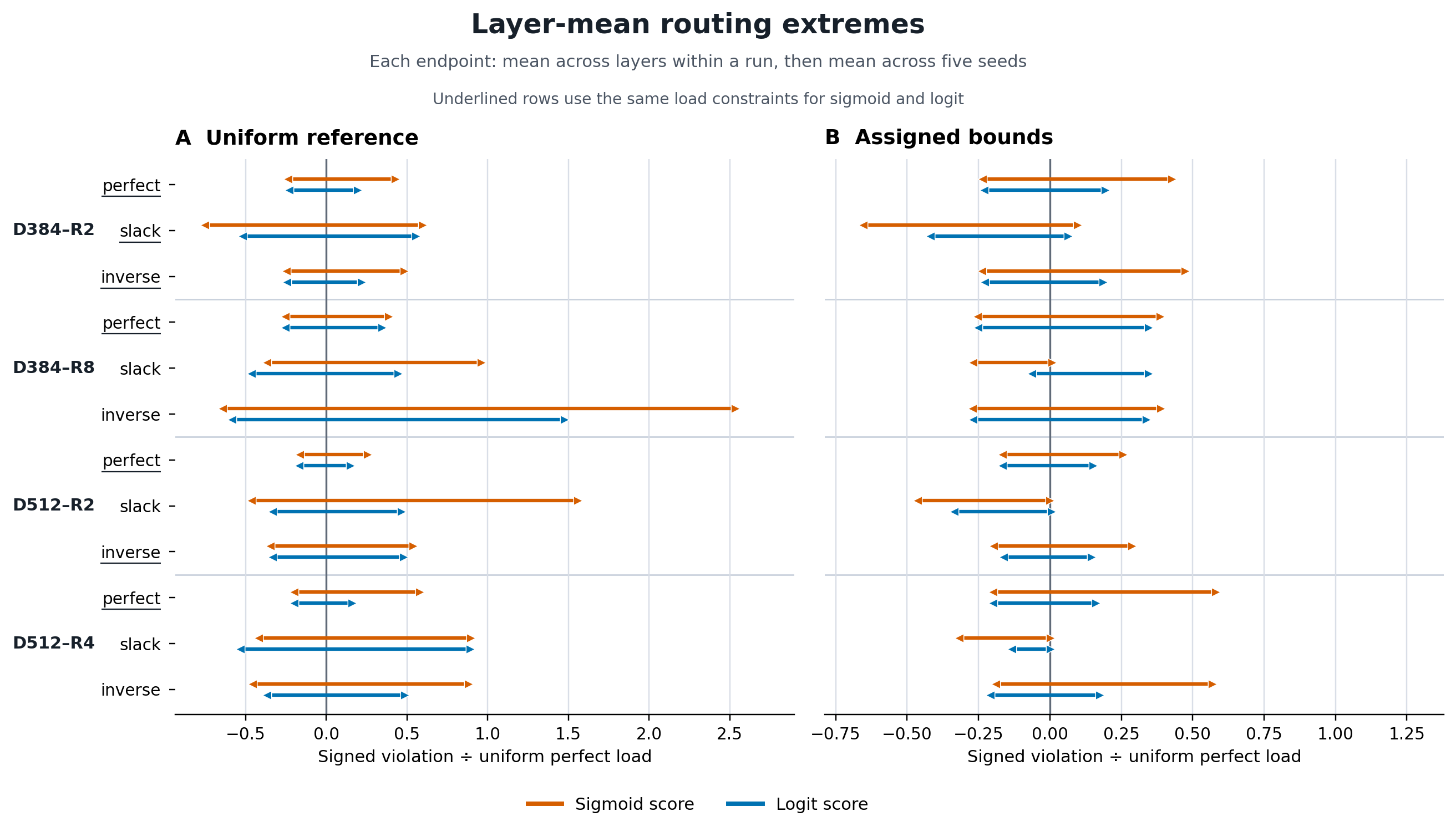
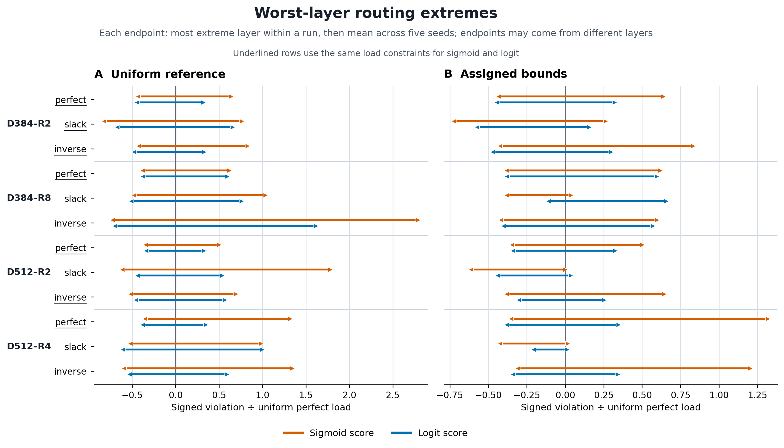
For loss, logit seems either comparable or better across all settings with perfect balance, but the story is a bit mixed across slack settings. So the primary benefit of logit seems to be better/more steerable balance (less violation of desired bounds) compared to sigmoid.
Relaxing exact load constraints
Now that we've considered the objective function, let's come to the constraints.
The constraints in quantile balancing are quite exact, and there is no way to control how strong the load balancing is. So this is a potential issue, especially if quantile balancing gives relatively good balance in an experimental setup (there are many important setups where it does not, so this needs to be considered, though it might be in some cases possible to fix those issues without relying on the load balancing algorithm as a crutch, e.g. by better depth scaling and router optimization, as here). As discussed in the previous section, perfect balance is not really needed if things such as MoonEP can reduce the serving/training penalty of not having perfect balance. There are at least two orthogonal-looking ways of deviating from uniformity - either we give experts some slack, or assign exact loads that are not uniform. The former might be more unpredictable, but for the latter, under perfect balance, it is possible to statically allocate experts and have load balancing across different ranks, if the exact load assignment is chosen appropriately (there is a wide range of choices that lets this work).
One intuition is that a model learns "greedily" at each step, which may lead to feedback loops leading to expert starvation. Load balancing tries to force it to have a good balance, because in the longer term it may be better to share capacity across experts. One of the predictions we can make is that for extremely sparse MoEs, a lower bound on the expert load is much more important than upper bounding. Controlling the slack we give to these bounds (or controlling the deviation from uniformity) can be a good way to balance the model's greedy choices with the model's long term health/training performance (and also load-balance-wise and loss-wise optimality). It could even be possible to schedule this rather than have it be static, but this would be quite complicated so we don't pursue this idea further.
So we try the following two things: first, instead of load being exactly , we assign bounds and where and (to see if we benefit from slack), and second, we assign non-uniform loads proportional to for expert rank , with for a tuned multiplier on top of the total number of routed experts and appropriate rounding (to see if we benefit from a certain non-uniform load distribution). The goal is to check whether this translates to loss improvements.
Does load slack improve loss?
We see that slack tends to help compared to enforcing perfect balance via quantile balancing, as far as loss goes.
Full slack comparison table
| Architecture | Router | Selected | Perfect loss | Slack loss | Slack minus perfect [95% interval] | Mean U Max/Min | Worst U Max/Min | Mean B Max/Min | Worst B Max/Min |
|---|---|---|---|---|---|---|---|---|---|
| D384-R2 | sigmoid | 2.901449 | 2.898040 | -0.003409 [-0.006757, -0.000061] | (+0.5968, -0.7538) | (+0.7627, -0.8260) | (+0.0979, -0.6538) | (+0.2628, -0.7259) | |
| D384-R2 | logit | 2.900888 | 2.898441 | -0.002448 [-0.004894, -0.000001] | (+0.5575, -0.5195) | (+0.6556, -0.6748) | (+0.0652, -0.4194) | (+0.1556, -0.5748) | |
| D384-R8 | sigmoid | 2.844130 | 2.841212 | -0.002918 [-0.004402, -0.001434] | (+0.9616, -0.3694) | (+1.0347, -0.4823) | (+0.0083, -0.2694) | (+0.0374, -0.3823) | |
| D384-R8 | logit | 2.842805 | 2.842229 | -0.000576 [-0.001389, +0.000236] | (+0.4470, -0.4627) | (+0.7575, -0.5107) | (+0.3470, -0.0635) | (+0.6575, -0.1107) | |
| D512-R2 | sigmoid | 2.834531 | 2.833618 | -0.000913 [-0.003746, +0.001920] | (+1.5599, -0.4643) | (+1.7797, -0.6137) | (+0.0000, -0.4642) | (+0.0000, -0.6137) | |
| D512-R2 | logit | 2.829211 | 2.827550 | -0.001661 [-0.003429, +0.000107] | (+0.4685, -0.3350) | (+0.5343, -0.4402) | (+0.0064, -0.3350) | (+0.0349, -0.4402) | |
| D512-R4 | sigmoid | 2.807199 | 2.804404 | -0.002795 [-0.006396, +0.000806] | (+0.8959, -0.4180) | (+0.9817, -0.5244) | (+0.0022, -0.3179) | (+0.0160, -0.4244) | |
| D512-R4 | logit | 2.804300 | 2.801389 | -0.002911 [-0.004233, -0.001588] | (+0.8917, -0.5328) | (+0.9953, -0.6079) | (+0.0016, -0.1328) | (+0.0126, -0.2079) |
The selected values of (and relative performance of other runs) show that it seems generally more important to keep the lower bounds somewhat tight while the upper bounds might be relaxed, especially for very sparse MoEs. The idea is that for very sparse MoEs, it is much more important to avoid underloaded experts (perhaps more learning signal is the bottleneck for these experts) than to tightly constrain the upper bounds on the load (which also gives evidence for the idea that a single shared expert might not be the optimal way to model high frequency experts).
Do inverse-rank load targets help?
We don't see a clear general benefit (and it doesn't harm loss either), so it does not seem that enforcing a distribution improves (or worsens) the loss as compared to perfect balancing. So it is possible that having slack matters more than an exact distribution, but I would also expect this setup to be at least slightly more sensitive to hyperparameters than the slack setup. Figuring out/learning the optimal exact distribution and/or its schedule (or in general, the exact lower and upper bounds), or further tuning, is out of scope, but could be worth trying.
Full inverse-rank comparison table
| Architecture | Router | Selected | Matching histogram | Perfect loss | Inverse loss | Inverse minus perfect [95% interval] | Mean U Max/Min | Worst U Max/Min | Mean B Max/Min | Worst B Max/Min |
|---|---|---|---|---|---|---|---|---|---|---|
| D384-R2 | sigmoid | compact | 2.901449 | 2.902396 | +0.000948 [-0.000759, +0.002655] | (+0.4829, -0.2467) | (+0.8263, -0.4272) | (+0.4743, -0.2377) | (+0.8323, -0.4249) | |
| D384-R2 | logit | relative-compact | 2.900683 | 2.900841 | +0.000158 [-0.001597, +0.001913] | (+0.2191, -0.2447) | (+0.3298, -0.4820) | (+0.1877, -0.2293) | (+0.2981, -0.4734) | |
| D384-R8 | sigmoid | compact | 2.844130 | 2.843212 | -0.000918 [-0.002940, +0.001105] | (+2.5337, -0.6420) | (+2.7900, -0.7285) | (+0.3898, -0.2724) | (+0.5968, -0.4187) | |
| D384-R8 | logit | relative-compact | 2.843154 | 2.841549 | -0.001605 [-0.004023, +0.000814] | (+1.4764, -0.5846) | (+1.6135, -0.7007) | (+0.3375, -0.2690) | (+0.5685, -0.4030) | |
| D512-R2 | sigmoid | compact | 2.834531 | 2.835464 | +0.000933 [-0.000640, +0.002507] | (+0.5387, -0.3491) | (+0.6932, -0.5208) | (+0.2876, -0.1983) | (+0.6442, -0.3816) | |
| D512-R2 | logit | relative-compact | 2.830004 | 2.829649 | -0.000355 [-0.002148, +0.001439] | (+0.4791, -0.3343) | (+0.5660, -0.4573) | (+0.1468, -0.1633) | (+0.2531, -0.3021) | |
| D512-R4 | sigmoid | compact | 2.807199 | 2.807132 | -0.000067 [-0.003003, +0.002868] | (+0.8834, -0.4579) | (+1.3415, -0.5962) | (+0.5686, -0.1891) | (+1.2025, -0.3103) | |
| D512-R4 | logit | relative-compact | 2.804427 | 2.803575 | -0.000852 [-0.005657, +0.003953] | (+0.4867, -0.3672) | (+0.5910, -0.5316) | (+0.1745, -0.2093) | (+0.3420, -0.3419) |
Alternatives to the quantile update
The remaining part is the actual algorithm being used to update expert prices. We've seen most of the relevant tradeoffs, so we will summarize those and talk about some in detail. We saw earlier how, under the same linear programming setup, aux-loss-free load balancing is a way to do gradient descent like algorithms on the dual and is quite cheap, but their step size doesn't handle the density of scores near the boundary, for which a Newton-like update could be plausibly thought of (though this problem is non-smooth, and needs approximation) - a diagonal Hessian-like approximation could be plausible. QB instead approximately solves each coordinate problem so it automatically adapts to such conditioning in some way, though it does not necessarily converge to an optimal solution. Optimizing using only a single batch's worth of data could also overfit on the batch and leave the estimate useless for the next update, so damping the update or checking whether the previous value gives a reasonable load or adding a proximal term that penalizes distance from previous parameter could help. These are relatively cheap and can be done using a histogram like standard QB. As we mentioned earlier, there seems to not be a good way of using stuff like bundle methods, ADMM, primal dual methods, LP/MCF solvers, Sinkhorn-style methods and so on, so currently there does not seem to be an obviously theoretically superior solver once training cost is taken into account, among the general purpose convex optimization solvers. Figuring this out could be interesting future work.
Acknowledgements
I would like to acknowledge various people in the Eleuther AI discord for discussing mixture of experts recently, GPT 5.6 Sol for writing up the outline section, creating images and writing most of the code.
References
- Conditional Computation in Neural Networks for Faster Models
- Outrageously Large Neural Networks: The Sparsely-Gated Mixture-of-Experts Layer
- Switch Transformers: Scaling to Trillion Parameter Models with Simple and Efficient Sparsity
- OLMoE: Open Mixture-of-Experts Language Models
- Mixture-of-Experts with Expert Choice Routing
- Hash Layers for Large Sparse Models
- DeepSeekMoE: Towards Ultimate Expert Specialization in Mixture-of-Experts Language Models
- Auxiliary-Loss-Free Load Balancing Strategy for Mixture-of-Experts
- Demons in the Detail: On Implementing Load Balancing Loss for Training Specialized Mixture-of-Expert Models
- MoE Travelogue 6: Optimal Assignment Promotes Balance (Quantile Balancing)
- MoE Travelogue 8: Enforcing Sequence-Level Balance (Moving Quantile Balancing)
- Kimi K3: Open Frontier Intelligence
- ZAYA1-8B Technical Report
- MAI-Thinking-1: Building a Hill-Climbing Machine
- Arcee Trinity Large Technical Report (SMEBU)
- REAP the Experts: Why Pruning Prevails for One-Shot MoE Compression
- MoonEP: A Perfectly Balanced Expert Parallelism Library via Dynamic Redundant Experts
- Megatron-LM baseline Quantile Balancing implementation, global-batch histogram implementation, and Kimi K3 support tracker
- Marin MoE experiment report
- The Myth of Expert Specialization in MoEs: Why Routing Reflects Geometry, Not Necessarily Domain Expertise.
Cite this post
@online{quantile-balancing,
  author    = {nor},
  title     = {Understanding, extending and improving quantile balancing},
  year      = {2026},
  month     = {09},
  day       = {02},
  url       = {https://nor-blog.pages.dev/posts/2026-09-02-quantile-balancing/},
}