Why wide neural networks share the same loss-curve fine structure
TL;DR
We start from a common empirical observation: when two sufficiently wide networks are trained on the same ordered sequence of minibatches, the small rises and falls in their loss curves can align almost step for step, even when their initializations are independent, and attempt to explain this in an elementary manner.
For a smooth two-layer network in the classical mean-field parameterization, trained for a fixed number of SGD steps, we show that for every fixed data stream , the vector of losses over steps differs from the deterministic infinite-width loss vector associated with by a vector whose RMS size is . The same conclusion holds after applying any fixed linear detrending operator .
If the examples used at every step are independent and the batch size is also allowed to vary, we show using another approach that, writing the finite-width loss vector in its two-factor Hoeffding/functional-ANOVA decomposition
where is the data-only component, is the initialization-only component, and is their interaction, under some smoothness and stability assumptions we get
Effectively, width averages over initialized neurons, batch size averages over examples, and the interaction is averaged over both axes. Consequently, same-data runs synchronize as width grows, while same-initialization runs synchronize as batch size grows.
These are pessimistic finite-horizon upper bounds for a smooth bounded two-layer model. Their constants depend on the training recipe and can grow poorly with the training horizon. Nevertheless, the rates match our empirical observations quite well, including in settings rather far from the one used for the proofs. There are papers using much heavier machinery that strengthen some of these results under different assumptions, but our point is that weaker but empirically useful conclusions already follow from elementary arguments.
Introduction
The Lean formalization of this blog's results can be found here.
If you've run multiple experiments while keeping the dataloader seed the same, you may have noticed something interesting: if you zoom into the loss curves, the short-timescale structure is quite detailed, and once the slow trend is removed, the rises and falls on short timescale can line up almost step for step, and this improves as networks get wider.
This is generally thought of as being driven by some sort of shared minibatch noise, but there are a couple of things that this understanding doesn't explain on its own:
- Why does the initialization stop mattering with width? Is this some kind of concentration effect?
- Why does the interaction between initialization and data ordering stop mattering too?
We will look at this for a smooth two-layer network in the classical mean-field parameterization, trained for a fixed number of steps with SGD. We will look at this only in the finite time limit, since this effect is quite visible during early training and it'll be easier to not worry about error accumulation as much.
A wide network is, in some sense, an average over many neurons. For a fixed sequence of minibatches, this becomes a Monte Carlo approximation to the infinite width case which corresponds to a full density over an infinite number of neurons (but this estimator is not necessarily unbiased).
So width averages over neurons, which reduces the initialization seed-specific error, while the variance due to the data still remains.
More specifically, we'll prove a bound of the following form, for a smooth two-layer neural network trained for a fixed number of steps using SGD:
with
where is the width, is the initialization, is the ordered data stream, is the vector of pre-update minibatch losses at each step. is the part that depends only on the data stream and other constants related to the training procedure (but not on width), and is the residual part, which we show is bounded in expectation. So the amplitude of the width-related noise decays as the width increases. To address the expectation over , we can use Markov's inequality to get (after making positive).
We will then also show that for mutually independent examples and under some other smoothness conditions, the data, initialization, and interaction components of the loss vector concentrate at the rates , , and respectively, in the sense (see the corresponding section for the exact statement). Here and later, hides constants that depend on the horizon , the training recipe, and the smoothness constants, but not on or - and as we discuss later, they can grow exponentially in .
While this doesn't give us a very general result that we can apply to standard transformer training (architecture/data/loss-wise), it gives us a toy model that can help us reason about this specific behavior, and also make some other predictions, like ones about detrended local loss curves, the kinds of concentration we can expect when scaling up training runs (and the acceptable noise in final loss values in scaling law predictions), and curricula. The bounds are also going to be (potentially extremely) pessimistic - and it seems to be a bad idea to trust pessimistic bounds in ML in general - but they give us some kind of guarantee on the concentration rates (where the exponents match empirical observations).
We first compare finite-width training with a true infinite-width trajectory for an arbitrary fixed data stream, and then use a different finite- argument to decompose and look at the data, initialization, and interaction effects.
Loss traces and the sources of randomness
Let's say we train the model for steps, and let be the loss at step . The loss trace corresponding to this run is the dimensional vector . For any trace (not necessarily just the loss vector), we say .
In a training run, there are two main sources of randomness: the initialization of the model, and the ordering (and contents) of the minibatches. We don't consider dropout/indeterminacy due to kernels/augmentation choices and so on.
We assume that, as usual, these sources are independent of each other. If we want to be pedantic, this may not hold if you've e.g. run data mixture experiments without reshuffling or without changing seeds, or other such things, but this is a reasonable assumption.
The first roadblock is that training couples the two and makes it hard to study them. We can still decompose the loss, however, as:
where , , , and .
Here the first term doesn't depend on anything, depends on the data stream only, depends on the initialization only, and depends on both (it is the part that can't be written as a function of data or initialization alone).
This is a two-factor Hoeffding/functional-ANOVA decomposition.
We have and .
As a result, the four parts of this decomposition are orthogonal in expectation (e.g., ), and we can write
How do we use this to think about the local loss?
Let's consider static detrending (not data dependent) - e.g., subtract a window mean from the current point. This is a linear transformation of the loss trace, and the detrended loss trace can be represented as for some matrix . Since is linear, it gives us a similar decomposition.
We can quantify the local similarity by detrending two loss curves and taking their cosine similarity or the L2 norm of their gap, which will be one of our points of focus.
The model
Consider a two-layer neural network with a single output, with width :
Here contains all the information about the -th neuron (e.g., for , and ).
The factor is the classical mean-field factor, and it's important because we will now interpret this neural network as a sample average. To do so, we will have to generalize things a bit.
Let's say the minibatch loss over a batch of size is , where . is a probability measure over "particles" .
Then the neural network corresponds to the empirical distribution , i.e., the particles are the neurons , and the empirical distribution is the mean of point masses (delta functions) over the neurons of the neural network. We can superscript these with to show that this is a given state of the neural network at step , as these particles evolve during training according to SGD.
In the feature learning regime, we want the "features" to evolve even in the infinite width limit. For any neuron, the gradients with respect to its parameters scale with , so the parameter-space learning rate should scale proportionally to , say at step .
Then a single step looks like
Here is the mean-field-scaled step size, and the scaled neuron update is:
Now let's see what happens in the infinite width limit. Let's fix a data order, say .
We have a distribution at step , say . To get to , we would sample from , apply , and see what the distribution of the mapped variable is.
The infinite width loss trace consists of , and this is the that we claimed earlier. Once is fixed, is deterministic.
What is held fixed when width and batch size change
In this parameterization the parameter-space learning rate is (while the "function-space" neuron update learning rate is around ). We keep the finite schedule and the horizon fixed as width changes. A nonconstant schedule causes no problem, but the constants in the bounds depend on the whole schedule. If the schedule itself changes with width, one needs uniform bounds on the resulting update maps.
The same issue appears when changing batch size. The rate below holds with the effective schedule fixed. If one tunes the learning rate as a function of batch size, the theorem can still be applied separately at every , but its constants now change with , so the observed scaling no longer isolates the averaging effect. Holding the schedule fixed is most plausible near or above the critical batch size, and less so in the regime where linear batch-size learning-rate scaling is useful.
For simplicity, the model in the proofs has no weight decay. A fixed smooth particle-level drift can be added without changing the argument. With decoupled weight decay applied directly to these particle parameters and the raw learning rate , keeping the particle-level decay fixed requires the raw decay coefficient to scale as . Other parameterizations need the analogous translation to an effective update whose constants stay uniform.Fixed-data-stream analysis
Let's fix the batch size, learning rate schedule, the initialization distribution, and pretty much everything other than the width.
Theorem 1: fixed-stream width concentration
We assume some smoothness (Lipschitz) constraints on the neural network, as well as some stability constraints on the training process, to make our life easier:
- The neurons are initialized i.i.d. (and the inits don't depend on the data).
- , , and initial particles all lie in bounded sets.
- We use SGD as above, with a fixed nonnegative learning-rate schedule and a fixed number of steps .
- There is a common compact convex particle set that contains every finite-width/mean-field trajectory we consider up to time uniformly in and all supported data streams . There is also a convex prediction region containing every prediction and every line segment between predictions compared below, with the stated loss bounds holding throughout that region.
- The feature is differentiable in , and and its parameter gradient are bounded and Lipschitz on the region reached within the steps.
- The loss is differentiable in the prediction, the loss itself and its slope are bounded there, and the slope is Lipschitz over the predictions reached within the steps.
- The maps and , and the maps and , are jointly Borel measurable. This is only measure-theoretic regularity (technical detail that you likely don't need to worry much about); it is used to justify the expectations and the random-stream consequence.
Note that we don't need independence between batches, so it doesn't matter whether we do SGD, or random reshuffling per epoch, or even no shuffling.
Note that since we are in a finite time regime, this is quite reasonable to expect for a smooth model. We can imagine a two layer MLP with tanh activations, with MSE loss (which may seem unbounded, but under finite time, is not an issue under standard conditions).
Under these assumptions, there is a constant , independent of and uniform over the supported fixed streams , such that
The idea behind the proof is the following. Compare each actual neuron with an ideal infinite-width particle starting from the same initialization. Conditional on , the ideal particles remain independent (each one follows the same deterministic sequence of maps driven by the mean-field distribution). The prediction gap then splits into the error accumulated by the coupled dynamics and a centered average of independent ideal particles. The latter is an ordinary Monte Carlo term with variance . Smoothness gives a recursion for the expected squared particle discrepancy of the form . Since and is fixed, we get for a fixed time horizon, and smoothness of the loss gives the claim.
Proof
Let's write down the smoothness conditions first. Suppose there are constants such that , , , , and , over whatever we observe during the training run.
Also, the particles are sampled i.i.d. independently of the data.
Now, we try to compare the infinite width limit with the finite width limit. To do that, we pick a particle , look at the idealized particle (as done before), and look at their joint evolution.
We have and .
Conditional on the data stream , the ideal particles are independent and their distribution is .
Let's say the expected discrepancy between the particles at step (expectation over initialization) is:
We will bound the error using smoothness conditions, and then propagate the prediction error through one step of SGD, which will give us a bound on , and then use it to bound the loss error.
For input , we have
By our second assumption and the mean-value theorem, we have .
The expectation of the first term squared, conditioned on , can then be bounded by using Jensen's inequality.
For the conditional expectation of the second term squared, it is a conditional variance (divided by ), and hence is upper bounded by the second moment divided by , which is upper bounded by .
Now, using , we get that
Now, we consider the SGD update.
Let's look at . The unscaled term inside the norm, corresponding to , is . Adding and subtracting , we get bounds for that term being . By triangle inequality, we get an upper bound of .
Let be the difference . Then we have .
So we have .
Applying Cauchy-Schwarz to the second term, we get .
Squaring and using again, and taking conditional expectation over given , we get
where and . We can then unroll this recursion.
Note two things:
- For a fixed number of steps, even though the bound becomes exponential in , it gives a bound that depends inversely on . The error accumulation that leads to such an issue is also why our analysis may give us useless bounds for long training times.
- Our bounds are quite weak, e.g., one way to strengthen them is to use (and there are other issues such as applying loose global bounds).
Now, we want to see how loss behaves.
The mean value theorem with the loss derivative boundedness assumption gives , so . Squaring and taking the conditional expectation with respect to given , then using the prediction error bounds in terms of and the bound we have above, we get the desired
Corollary: detrending and same-stream loss synchronization
Now let's see what happens with a linear transform .
We have , so
Now using element-wise, for two independently initialized runs of widths and with the same data stream, we get
If is nonzero, the gap bound also gives in conditional probability as . The gap bound is a stronger and potentially more useful statement.
Let's look at the Hoeffding components again. Suppose now that the random-stream law is supported almost surely on the supported streams above (technical detail that you likely don't need to worry much about). If , then , , and in mean square, where the last two terms scale as (due to orthogonality and operator norms). Synchronization only needs the interaction and the initialization terms to vanish (which they do).
Some discussion is in order:
- This only considers upper bounds, and these are very strong conditions and the bounds we have are extremely pessimistic. One can still think about some of these inequalities being approximations (with smaller constant factors), and getting more realistic constants, but that is still not a proper proof. In fact, it is also possible that the rate is not tight, and that the convergence is even faster. However, Bordelon and Pehlevan (2023) do a sharper analysis of finite width corrections and get a similar rate. We also show this rate experimentally for our setting.
- There is a difference between two ideas - ensemble at a fixed width and the actual infinite-width limit. Our bound controls the total deviation and is dominated by initialization noise. Vyas et al. (2023) show empirically that after ensembling away this noise, a systematic finite-width bias remains. We do not resolve that smaller effect. This is one way in which the next section's approach differs from this section, where the reference is a finite-width ensemble rather than the mean-field limit.
- Unlike a gradient-flow argument, our discrete-time argument is not immediately incompatible with edge-of-stability behavior. However, its constants can grow exponentially with the number of steps and may become useless by the time progressive-sharpening finishes. It is possible that a different explanation dominates at such horizons, and I have not thought in more detail about this.
- Boundedness is used to keep all derivative constants uniform over the trajectories being compared. Projected methods can make this easier, though their boundary effects would need separate treatment. Weaker assumptions should also be possible, but the present ones make the main mechanism clear regardless.
Changing the batch size
In the previous section, we fixed and got the regime where the data dependent loss fine structure can survive as width goes to infinity. If we increase , we should expect the data component to concentrate too. Scaling width reduces the randomness due to sampling finitely many neurons at init, while scaling batch size reduces the randomness due to sampling finitely many examples (and their interaction is affected by both).
The two results use different comparisons, and neither is just a corollary of the other. The first allows an arbitrary fixed or reshuffled stream and compares a finite network with its true mean-field limit, but says nothing about varying . The result below assumes independent examples and stronger smoothness, and compares a run with finite- ensemble means rather than with an infinite-width trajectory.
Let's first look at what happens when there is no training, i.e., before the first step.
Let denote a random example, and let be the single-sample loss.
The infinite-width minibatch loss before any update is . Since the -s are i.i.d., the variance of is exactly times the variance of .
Now when there's training, an example affects both the current loss as well as the loss for subsequent steps.
We will make a stronger assumption this time: all examples are mutually independent, and within each step they are identically distributed. The step- distribution may vary with , which allows for using fixed randomized curricula. The argument below doesn't directly handle the more commonly used random reshuffling without replacement, and it would need some more work.
Let be the loss trace, where and . We use the same finite-size Hoeffding decomposition:
The components are defined at the actual finite and (note that this is different from the previous section where we could use infinite width), with :
and .
In particular, the width- ensemble trace for a fixed stream is
so
Similarly, the data ensemble for a fixed initialization is
Unlike in the previous section, this is not the infinite-width limit: the systematic finite-width displacement of the ensemble mean is already inside .
Theorem 2: two-factor (minibatch and initialization) finite-size concentration
Under the assumptions in the proof below, there are constants independent of and such that
where .
The first two rates are what we would expect from averaging neurons and examples separately. The last rate gives us a concrete higher-order term averaged over both axes.
The proof idea is to replace one initialized neuron, one training example, or both by independent copies. Stability and the two averages in the update give deterministic influence bounds of , , and on the whole loss trace. Efron-Stein then squares and sums these influences over neurons, examples, or all neuron-example pairs. This gives second moments of order , , and respectively.
Proof
Write one SGD update as
where
and . The prediction at a particle configuration is
The loss before the update is
Thus, if is the batch at step , then
where denotes one SGD step, and
The full loss trace is
and we use the usual Euclidean norm on traces:
Let's first write down the assumptions:
- The number of steps and the nonnegative effective learning-rate schedule are fixed as and change, as discussed in the parameterization section above. In particular, increasing also increases the total number of examples used.
- The initialized particles are i.i.d.
- The examples are mutually independent and independent of the initialization. Within step they are identically distributed according to , but may vary with .
- The initialization and data distributions have bounded measurable support, and the selected support sets have probability one.
- There is a fixed compact convex set containing every particle state reached during the first steps, including in the coupled runs used below.
- On this region, is differentiable in its particle argument, and its first derivative is bounded and Lipschitz.
- On the product of the particle and prediction regions, is differentiable in , its first Fréchet derivative is bounded and Lipschitz, and itself is bounded.
- The loss is differentiable in ; the loss and its slope are bounded over the prediction region, and the slope is Lipschitz there.
- The feature, feature-gradient, loss, and loss-slope maps are jointly Borel measurable in their arguments, so the trajectories, traces, and expectations below are measurable.
All derivative bounds below are understood to hold on a compact convex set containing the particle states and on a compact interval containing every prediction encountered in the coupled runs. Thus, every line segment used in the mean-value and fundamental-theorem-of-calculus arguments remains inside the region where the derivative bounds hold.
No differentiability with respect to the example is needed.
For convenience, choose constants such that
and the first derivatives of , , and are Lipschitz, with constants bounded by , , and .
We replace one initialized particle by an independent copy and get a new trace . Similarly, we replace one example and get a new trace . We then replace both and get a new trace .
Define
and
We will first prove that there are constants , independent of , , , , and , such that
and
For two particle configurations (neural network weights), define
and
The average norm is useful for a neuron replacement. Replacing one particle can change that particle by an order-one amount, but the average change over all particles is only .
The maximum norm is useful for an example replacement. Replacing one example changes the update of every particle by , so the perturbation is even in the maximum norm.
We first derive some basic stability bounds.
By the mean value theorem,
This gives
Now consider two configurations and updated using the same batch . For particle ,
Using the Lipschitz bound on ,
Using the prediction bound,
Averaging over gives
where we may take
with
Taking the maximum over gives
Both constants are independent of and . This comes from the two averagings: the prediction is an average over particles, and the update is an average over examples.
The corresponding same-minibatch loss bound is
Now suppose that batches and differ in exactly one example. Then, only one term in the update changes. Since ,
Similarly, only one term in the loss changes, so:
We also need to know how the effect of replacing an example changes when the particle configuration changes. Suppose again that and differ in one example. Applying the Lipschitz bound on to the replaced example and to its independent copy gives
where depends only on , , and .
The analogous loss bound is
We can now prove the first two replacement bounds.
First, replace one initialized neuron. Let's couple the original and perturbed runs so that they use the same data stream. Let their particle configurations be and , and define
At initialization, only one of the particles differs. Since is bounded, there is a constant such that
The two runs use the same batch at every step, so
Unrolling the recursion, we get
The loss difference at step is therefore bounded by
Hence
Since is fixed, the sum is a constant depending only on . Therefore there is a constant such that
Now replace one example .
The two runs have identical particle states until step . At the loss recorded at step , one of the loss summands changes, so
At the update at step , one of the update summands changes, so
The same bound also holds in the average norm.
For , define
and
After step , the two runs again use the same batches. The stability inequalities give
and
Therefore there is a constant such that
Since , it follows that for some constant ,
for every , by unrolling the recursion.
At later steps, the two runs use the same loss batch, so
Combining this with the direct change at step , there is a constant such that
Now it remains to prove the mixed replacement bound
We first record a deterministic second-order difference lemma.
Rectangle lemma. Let , where is convex. Suppose
and
For four points , with , define
and
Then
where depends only on the derivative bounds and on the compact domain containing the four points.
To prove this, write
Then
By the fundamental theorem of calculus,
and
Subtracting these expressions and adding and subtracting gives
The first integral has norm at most . For the second integral,
Since , the second integral is bounded by
The four points lie in a fixed compact set, so is uniformly bounded. The term can therefore be absorbed into the coefficient of , which proves the lemma.
We now apply the lemma to four coupled training runs. Write their particle configurations as
where means that initialized neuron was replaced, and means that example was replaced.
For each particle , define its rectangle difference by
Also define the particlewise one-factor perturbations
and
At the configuration level, define
and
The one-neuron and one-example arguments already give, uniformly for and after enlarging and if necessary,
We also have
because the maximum of two nonnegative quantities is at most their sum, and
for every particle .
We first control the corresponding rectangle difference of the prediction.
For a fixed input , define
Since
applying the rectangle lemma to the map particle by particle gives
After changing the constant, we may write this as
The corresponding first-order prediction differences satisfy
and
The first inequality follows from the average norm. For the second, note that
Now suppose that all four runs use the same batch
For an example , write
For particle , apply the rectangle lemma to the map
at the four points
The rectangle difference of these four input points is
Their differences in the initialization direction are bounded by
and their differences in the example direction are bounded by
Consequently,
The average of the product term is bounded by a constant times . Indeed,
Here we used
as well as
Together with the prediction rectangle bound, this gives
uniformly in .
The update map contains the identity map and an average over the batch. It follows that
Using , there are constants and , independent of and , such that
whenever all four runs use the same batch.
The loss obeys an analogous rectangle bound. Applying the rectangle lemma to the map
for each example and then averaging over the batch gives
It remains to handle the step at which the replaced example first appears.
Before step , changing has no effect. Hence, for each ,
Write this common state as . In particular,
Let the original and replacement examples be
For one example, define the vector-valued map
The Lipschitz bounds for and the prediction imply
At step , only one of the update summands differs. Therefore
The mixed loss difference at step is also controlled directly. All unchanged summands cancel, leaving
After step , the four runs again use the same batch at every step. Hence,
The one-factor replacement bounds give
Starting from , we obtain, for ,
Since is fixed, the expression in parentheses is bounded by a constant depending only on and the smoothness constants. Thus,
for every .
For , the mixed loss difference is zero. At , it is bounded by by the direct calculation above. For , the common-batch loss rectangle bound gives
Therefore every coordinate of the mixed trace difference is bounded by . Consequently,
Absorbing the fixed factor into the constant gives
Together with the previously established bounds
this proves the three deterministic replacement bounds.
We now turn them into bounds on the Hoeffding components.
Recall that
and
We use the vector Efron-Stein inequality. If a random vector depends on independent random variables , and is obtained by replacing by an independent copy, then
First consider , which depends only on the initialization.
Let be obtained by replacing initialized neuron by an independent copy. Then
Applying Efron-Stein over the initialized neurons and then conditional Jensen gives
Next consider , which depends only on the data stream.
Let be obtained by replacing example by an independent copy. Then
There are independent example coordinates. Applying Efron-Stein over them and then conditional Jensen gives
Finally consider the interaction . For every fixed data stream , has conditional mean zero over . We may therefore apply Efron-Stein over the initialized neurons conditionally on , and then average over as follows:
The term depending only on the data stream cancels when initialized neuron is replaced. The remaining difference is
For fixed and , define
This random vector has conditional mean zero over the data stream. Applying conditional Efron-Stein over the independent example coordinates gives
The centering term does not depend on the realized data stream, so
Substituting this conditional bound into the first Efron-Stein inequality gives
Taking square roots gives
and
Therefore, for fixed (and under our original assumptions),
Consequences of the two-factor decomposition
The same result holds for any fixed linear detrending operator , with every RMS bound multiplied by . Thus the batch-size conclusion applies directly to local loss traces as well.
Let for . These latent component variances can be recovered from observable raw-run contrasts. For independent copies of every resampled factor, define
and
ANOVA centering and orthogonality give the exact identities
Consequently,
The finite-size bounds imply
Again, these are upper bounds, and e.g., don't say that the leading coefficients are nonzero. At initialization, however, the scaling can already be seen from a first-order expansion. Let
and define
For , take the step-zero example law . The initial minibatch loss has the following exact decomposition:
where, if ,
The local Taylor theorem on the prediction interval gives the rigorous bound
Since for every supported , the first three terms are a data average, a neuron average, and a degenerate two-way average. After subtracting the common mean from the data average, their second moments are exactly their respective population second moments divided by , , and . Consequently their RMS values scale as , , and whenever the corresponding population variances are nonzero. The bounded supports, bounded prediction region, local loss bounds, and joint Borel measurability assumed above ensure these moments and conditional integrals exist; no separate integrability premise is being hidden here. This is only meant to show that the leading coefficients can already be nonzero at , it is not a uniform joint expansion in and , and says nothing directly about later steps. The finite-time result above supplies the upper bounds during training.
There are three useful limits:
- With fixed and , and vanish, while may remain. This is the loss-synchronization regime.
- With fixed and , and vanish, while initialization variation may remain.
- If both grow, all three centered random components vanish at the upper root-mean-square rates above.
Another interesting thing is that if you remove from to get , we can define normalized shared-factor covariances (where and are independent copies):
Then we have
The remaining fraction is the interaction term.
To make the approximation precise, suppose that for some additive remainders
Set
If and , then the actual variance denominator is positive and
and
Thus, when the scaled additive remainders are small relative to the leading denominator, the amount of shared variation is quantitatively close to the expression controlled by the ratio of batch size and width. Without such remainder control, the upper bounds alone do not justify the displayed leading-order fractions.
There is also the same time-horizon caveat as before. The proof repeatedly multiplies worst-case Lipschitz factors, so can grow exponentially and become practically useless. The rates in and , however, are still remarkably robust.
Implications
As earlier, one should remember that this is only a toy model, but we should expect some implications to transfer.
The deterministic influence bounds in the previous section also give conditional versions of the synchronization statements. Uniformly over a fixed supported data stream ,
and uniformly over a fixed supported initialization ,
Thus training runs with the same data but different initializations synchronize as width grows, while runs with the same initialization but different data synchronize as batch size grows.
Also, due to the rectangle analysis, at sufficiently large and , the effect of changing initialization becomes nearly independent of the data. And the results we obtained also give evidence for usefulness of tricks such as debugging initialization by using large batches, and (the not-so-common) studying data by using wide networks (under the assumption that things stay stable even after scaling up).
For a fixed scalar statistic (e.g., final step loss or fixed window average for the last window), , there is a factor of in the bounds, which indicates that averaging across steps can reduce variance in results (but isn't really a proof since other constants can change).
For scaling law runs (with the caveat that this corresponds to training loss instead of validation loss), if the step count is kept the same (unrealistic considering typical batch size scaling laws are sublinear in total tokens, but let's assume this for now), then these results can help be more confident about the typically expected variance (such a variance would also follow a scaling law that can be empirically fitted too), instead of often reported ungrounded measures such as percentage points of loss. It is also worth thinking about what happens when noise can prevent us from measuring scaling improvements cheaply. Let's say our compute scaling law is for an exponent and compute . Let's say the single run variance is . If we use a compute multiplier of , the expected improvement is proportional to , and the single run SNR is proportional to . If this SNR decreases with , then gains become harder to figure out at scale.
Note that the results are still valid when the per-step data distribution is different for different steps. So a fixed curriculum can still be somewhat modeled using this method. It might be possible to think of the data effects in a hierarchical manner - a random curriculum plus within curriculum randomness, and do a similar bounding with three-factor Hoeffding/ANOVA (though it would still be pessimistic).
Experimental results
Measurement and fitting
Details
For every condition, the raw observation was a pre-update loss trace , with initialization and ordered minibatch stream fully crossed. We report magnitudes using the time-averaged norm
For synchronization, subtracts a centered 21-step moving average (ten steps on either side), using only the available points near the boundaries. For each stream, we average the widest reference networks over initialization to get , and measure
These are wide but finite numerical references, not the infinite-width solution.
The variance components use the standard correction for a crossed random-effects design. Let , , and be the initialization, stream, and grand means, and let
We compute
and use the signed estimates
The plotted component magnitudes are the square roots of the positive estimates.
Exponents come from a rank-weighted least-squares fit of , with ranks giving moderately more weight to the larger-scale points. The two-coordinate interaction fit uses and the product of the width and batch-size ranks. The gray lines in the figures are visual references to compare slopes.
We do 1,000 crossed-factor bootstrap resamples and look at intervals (accounting for initialization and data sampling).
The controlled experiments supports this reasonably well, and intervals from the optimizer experiments are more like sanity checks.Controlled simulation
First we check if the scaling exponents are indeed correct for our special case (single-hidden-layer mean-field network with SGD) in the average case instead of just in the worst case.
We note that the raw loss curves approach the fixed large width loss curve as width increases, and after the fixed detrending operation is used, we see local alignment between loss curves even at small widths, while the initialization-specific deviations reduce with width.
Estimating the RMS magnitudes of , , and , we get exponents remarkably close to the predicted ones (usually within , and within in the worst case), with reasonable factor-bootstrap intervals. So we move on to harder and slightly more diverse cases.
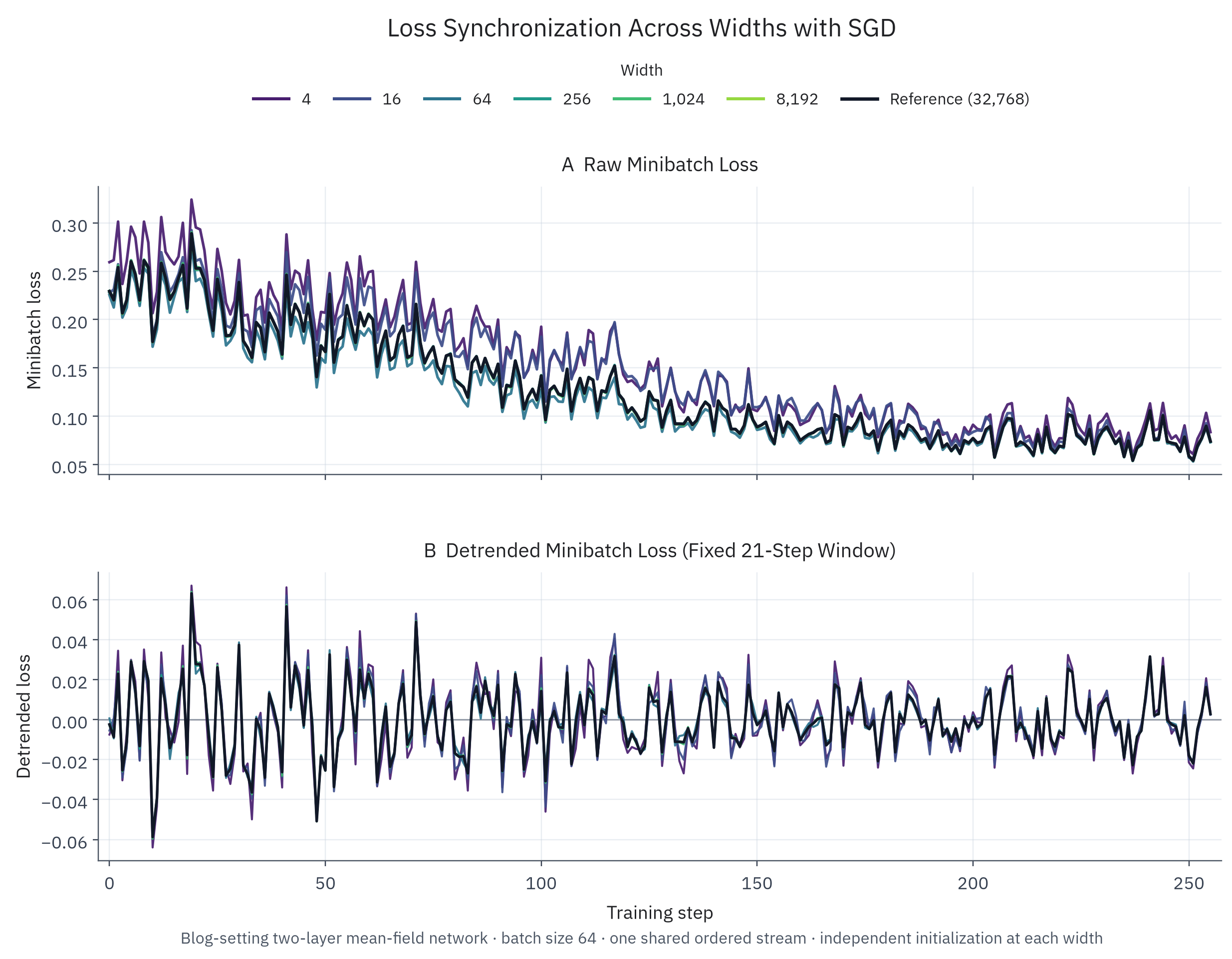
Details
The particle learning rate for SGD was (so the raw learning rate was ), the training horizon was steps, the batch size was , the inputs were uniform on , and the function to be learnt was
A grid of initializations and i.i.d. fresh minibatch orders was used (and initializations at different widths were independent).
The conditional mean of 6 i.i.d. width- networks was used as a finite reference for each stream.
Figure 1 uses a particular shared data stream, while the estimates use the full grid.
The synchronization and component width fits at batch size use widths through . The data batch-size fit uses batches through at width , and the initialization fit uses widths through at batch size .
Validity beyond the two-layer model, and beyond SGD
We want to check whether the phenomenon is more general (and whether our exponent upper bounds are tight in other scenarios too).
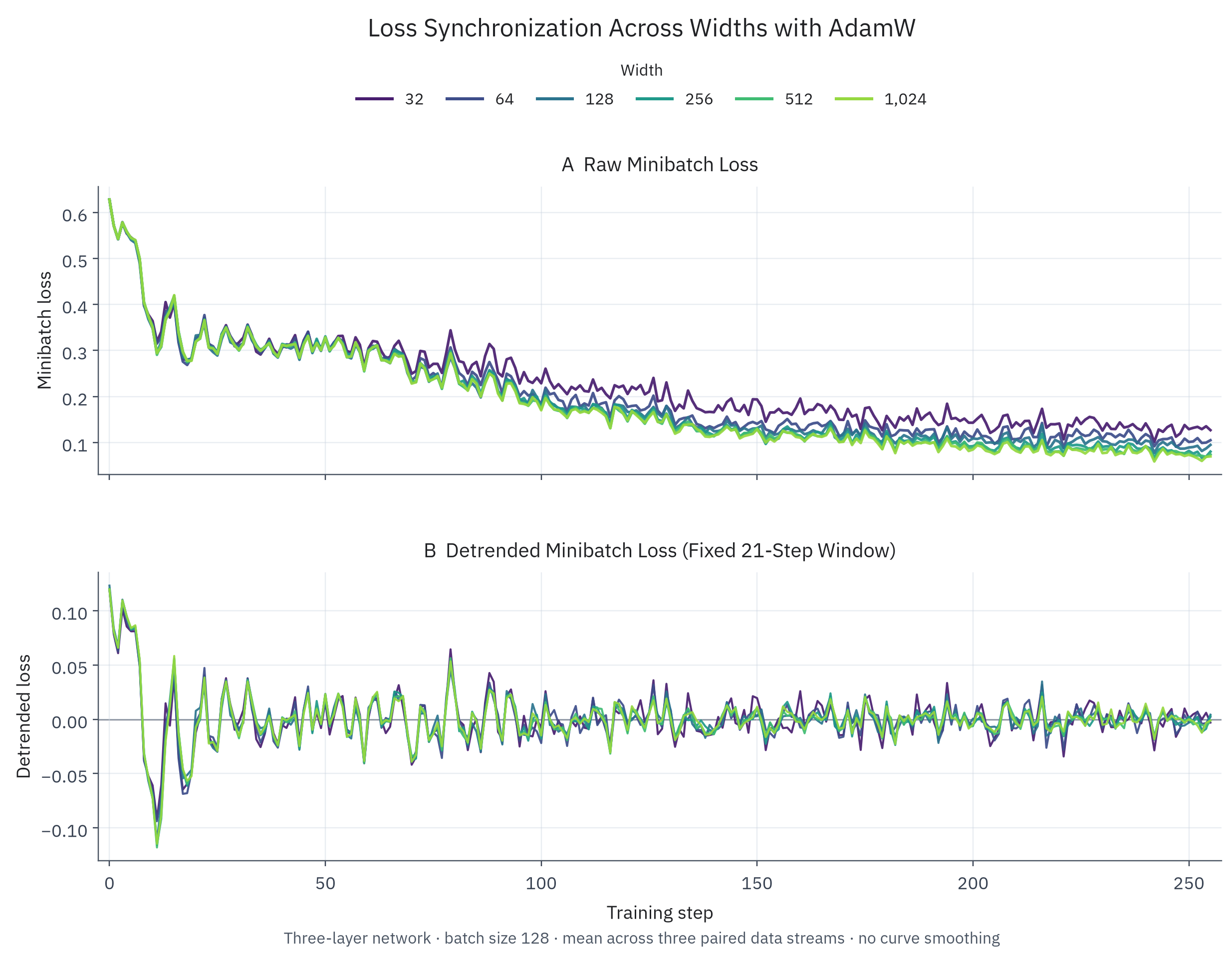
We choose a two-hidden-layer model (MLP with two tanh layers) with three optimizers - SGD with momentum and weight decay, AdamW, and Muon (with weight decay) - all with a linear-to-zero LR schedule, tuned according to loss and transferred using their appropriate P parameterizations.
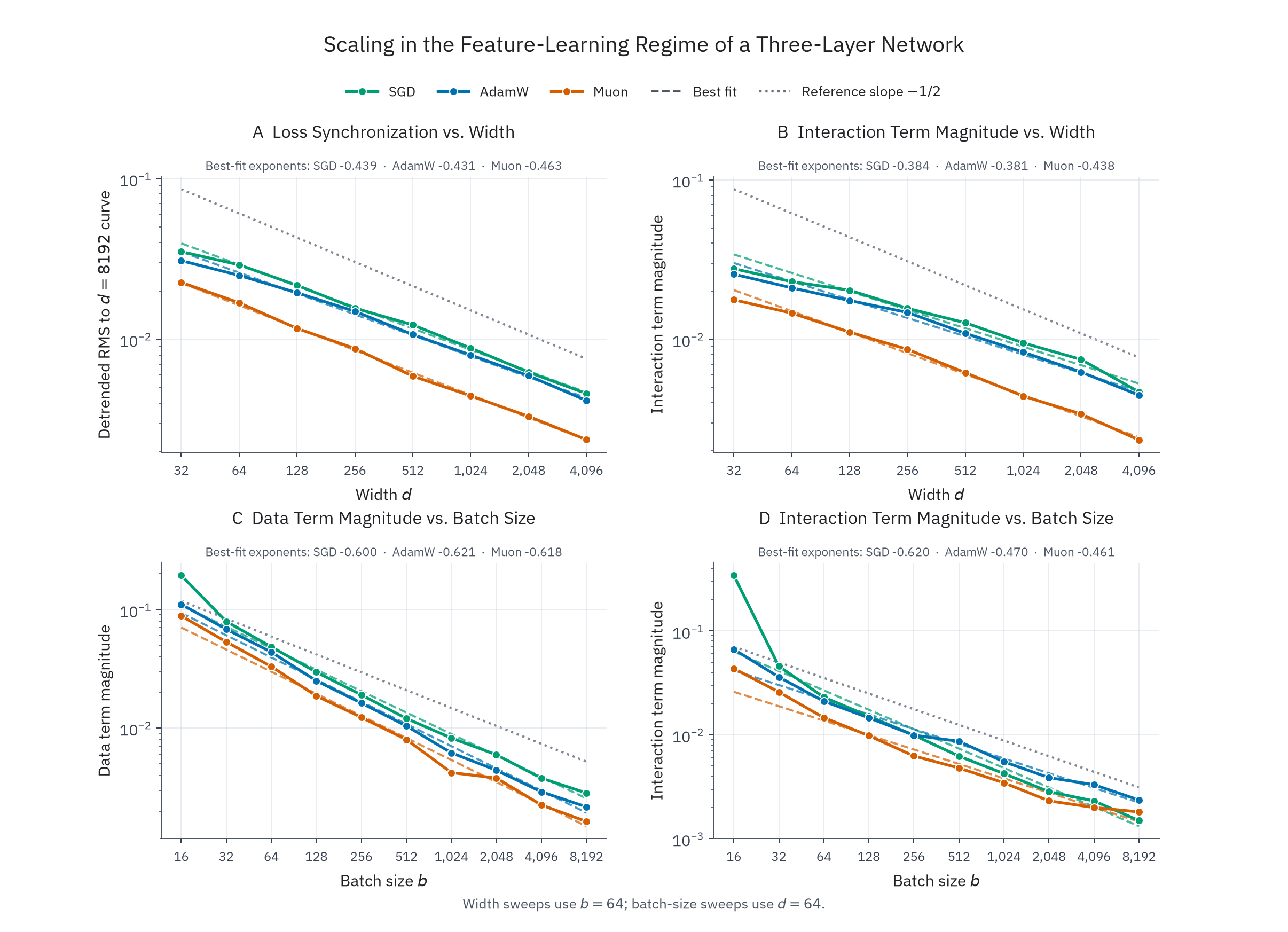
Figure 2 shows concentration for AdamW for a pre-tuning run in the setup, and Figure 3 shows the results of fitting rates for the complete experiment.
We find a reasonable match between the rates derived for a single-hidden-layer mean-field model with SGD and the empirical exponents for these three optimizers on a different model.
Details
We use the same initialized parameters and (more complex) i.i.d. data streams for all three optimizers (4 initialization seeds and 4 data seeds). Every run had 256 steps. Width ranged from for measuring width effects at batch size , and batch size ranged from for measuring batch-size effects at width . The width- reference averages four initializations separately for each stream. The width fits use all eight finite-width points, and the batch-size fits use all ten batch sizes. Because there are only four levels of each crossed factor, the component intervals here are primarily sanity checks.
Related work
Vyas et al. (2023), Feature-Learning Networks Are Consistent Across Widths At Realistic Scales study agreement of early loss curves, predictions, and representations across widths and study both initialization variance as well as a systematic narrow-ensemble-infinite-width gap. Their initialization-dependent prediction variance scales as , or in root mean square. They also find an bias rate.
Bordelon and Pehlevan (2023), Dynamics of Finite Width Kernel and Prediction Fluctuations in Mean Field Neural Networks use dynamical mean-field theory to study fluctuations more precisely. They characterize fluctuations of kernels, predictions, and order parameters, corresponding to variances, and they include discrete-time large-learning-rate effects. The elementary proof here does not recover their precise conclusions.
The fixed-data analysis uses mean-field and propagation-of-chaos arguments. Relevant results include Mei, Misiakiewicz, and Montanari (2019), Mean-field theory of two-layers neural networks: dimension-free bounds and kernel limit and De Bortoli et al. (2020), Quantitative Propagation of Chaos for SGD in Wide Neural Networks (in continuous time, instead of discrete time SGD). Earlier particle and fluctuation viewpoints include Rotskoff and Vanden-Eijnden (2018), the law-of-large-numbers and central-limit work of Sirignano and Spiliopoulos (2020), and the finite-time dynamical CLT of Chen et al. (2020).
The poor step-count dependence of our proof is not something that is always going to be true. Glasgow, Wu, and Bruna (2025) obtain propagation-of-chaos control beyond logarithmic time in a certain feature-learning problem, and Guillin, Nectoux, and Stos (2026) prove uniform-in-time concentration for a quadratic-loss, ridge-regularized two-layer setting. These works rely on stability or regularization structure absent from the general bounded-Lipschitz estimate here.
The minibatch fluctuation literature is directly relevant to the second theorem. Descours et al. (2024), Law of Large Numbers and Central Limit Theorem for Wide Two-layer Neural Networks: The Mini-Batch and Noisy Case prove trajectorial law-of-large-numbers and central-limit results and study how minibatching contributes to the limiting fluctuation variance. Descours et al. (2026), Quantifying Uncertainty in Wide Two-Layer Neural Networks characterize the limiting Gaussian fluctuation process and its covariance in a related regime. The distinct emphasis in the post is the finite-size two-factor Hoeffding/functional ANOVA, the mixed replacement bound, and the resulting experimental identities for loss traces.
For scaling-law implications, Kaplan et al. (2020) give the early nearly-constant-serial-step prediction (which turns out to be incorrect), while Hoffmann et al. (2022) revise the compute-optimal allocation between model size and tokens. McCandlish et al. (2018) introduce the critical-batch framework; Zhang et al. (2024), Li et al. (2025), and Schaipp (2026) study modern batch-size and step-count scaling. Porian et al. (2024) and Choshen, Zhang, and Andreas (2024) explicitly discuss loss noise and seed variability in scaling-law estimation.
Acknowledgements
GPT 5.6 Sol helped in checking the math in parts of this post, formalizing in Lean/expanding upon some arguments, writing experiment code, as well as polishing prose and helping with LaTeX. After my first draft, it also found all the related literature that is cited above. Responsibility for the claims, their correctness and references remains with me.
WhereIsTheExit read through a first draft of the post and gave helpful comments on readability.
Cite this post
@online{wide-loss-fine-structure-2026,
  author = {nor},
  title  = {Why wide neural networks share the same loss-curve fine structure},
  year   = {2026},
  month  = {07},
  day    = {12},
  url    = {https://nor-blog.pages.dev/posts/2026-07-12-why-wide-neural-networks-share-the-same-loss-fine-structure/},
}