Deriving RoPE the proper way

Figure 1: Attention score similarity with our 3D RoPE. These plots show how positional similarity changes across an axis.

Introduction

RoPE has become the de facto positional embedding for transformer models. Its popularity mainly stems from its performance, but the “derivation” in the paper is also quite elegant (but flawed).

Implementing high dimensional RoPE also pushes us to think about generalizing the underlying ideas as much as possible (alongside using signal processing intuition) - there’s code at the end of the post that implements things based on the ideas we develop here.

Upon a closer look, the original derivation is unfortunately not rigorous - the paper solves the problem for 2 head dimensions (not position dimensions), and then proceeds to generalize it to a higher number of (even) dimensions with a similar-looking form. That does provide a solution, but is still incomplete in terms of whether or not there are other solutions. There is another attempt at proof here that talks about completeness, but it makes some assumptions, while being accidentally benign, that leave the proofs incomplete.

So I decided to settle this question, and show that RoPE is actually optimally expressive under these conditions. Well, not quite - a couple of little things make it slightly suboptimal, but increasing the head dimension just works.

And as a bonus, we find how to generalize standard RoPE to $N$ dimensions for free. Then we show a general construction that guarantees quality-related properties such as incoherence and quality.

The Problem

The setting is the following.

You want to encode the position of each token somehow. In a transformer, to compute the attention scores, we compute the query $q$ and key $k$, and then take a dot product. The question we ask is the following: can we replace them by $f(q, p_q)$ and $f(k, p_k)$ such that some nice properties hold?

Let’s think about these properties. Since the actual position in the text really doesn’t matter when we look at two tokens, we want this product to be solely a function of $q$, $k$ and $p_k - p_q$.

Also, it is reasonable to assume that the norm of the embedding doesn’t change after performing this encoding, i.e., $||f(x, p)|| = ||x||$. $f$ still has a large space of solutions, so we want to restrict it to linear transformations, i.e., $f(x, p) = M(p) x$ for some function $M$ that maps positions to matrices with size compatible with $x$. And it doesn’t hurt to assume that $M(0) = I$.

The Solution

This is a functional equation for $M : \mathbb{Z}^n \to \mathbb{R}^{d \times d}$, where $n$ is the number of dimensions (i.e., our positions are in an $n$-dimensional integer lattice), and $d$ is the dimension of the attention head. Note that we could have also solved the problem on $\mathbb{R}^n$ instead of $\mathbb{Z}^n$ but it requires some further assumptions for non-absurd solutions (and is hence delegated to the next section).

We need $\langle f(q, p_q), f(k, p_k) \rangle = g(q, k, p_k - p_q)$.

Norm preservation gives $M(p)^T M(p) = I$, so $M(\cdot)$ is orthogonal. (Note that norm preservation is not really necessary, the line below for $p_q = p_k$ and $M(0) = I$ lead to this property already).

The original equation gives that $M(p_q)^T M(p_k)$ is a function of $p_k - p_q$, let it be $H(p_k - p_q)$.

Plugging in $p_q = 0$, we get $M(p_k) = H(p_k)$. Then using orthogonality, we have $M(p_k) = M(p_q) M(p_k - p_q)$. By a simple change of variables, we see that $M$ satisfies $M(a + b) = M(a) M(b)$.

Note that $+$ is commutative, so $M(b) M(a) = M(b + a) = M(a + b) = M(a) M(b)$. This gives us a very strong result: all the $M(⋅)$-s commute.

Also, note that $M(p) M(-p) = M(0) = I$, so $M(-p) = M(p)^{-1}$. Using this and letting $e_i$ be the standard basis vectors for the lattice, we get $M(p) = M(\sum_{i} p_i e_i) = \prod_i M(e_i)^{p_i}$, even for negative $p_i$.

So all that remains is to characterize $M(e_i)$. Call that $M_i$. Now these matrices all commute with each other, and are orthogonal. Then by the spectral theorem on commuting families of real orthogonal matrices (can be found e.g. as Corollary 2.5.11(c) in Horn and Johnson’s Matrix Analysis), there is a $P$ that simultaneously block diagonalizes all $M_i$. And these block diagonal matrices have the same block structure - $2 \times 2$ matrices first, then $1 \times 1$ matrices. The $2 \times 2$ matrices are rotation matrices, and the $1 \times 1$ matrices are all $± 1$-s.

Now combining this, we get $M(p) = P \left( \prod_i M_i^{p_i} \right) P^T$.

Now let’s see how to reduce this to RoPE (well, almost).

Firstly, we can get rid of $P$ and $P^T$. To see this, note that $f(q, p_q) = M(p_q) q = P M’(p_q) P^T W_Q x$ (where $M’$ is the block diagonal function), so we can absorb $P^T$ into $W_Q$ (to a matrix $W_Q’ = P^T W_Q$). Do the same for $W_K$. To get rid of the $P$, note that $f(q, p_q)^T f(k, p_k) = x^T W_Q’^T M’(p_q)^T P^T P M’(p_k) W_K’ x = x^T W_Q’^T M’(p_q)^T M’(p_k) W_K’ x$, where the $P$ vanishes due to orthogonality. So we can safely ignore that and just learn $M’(p)$.
All that remains is that we remove the $± 1$-s from the expression. If there are $k$ of these terms, then we can just duplicate these one by one on the diagonal to make $2 \times 2$ block matrices on the diagonal (since these correspond to rotation by $\pi$ or by $2\pi$, of the vector $[\cdot 0]$ if the element is $\cdot$), while adding 0 projections to the original $q$ or $k$ vector in the corresponding dimension (this can be done by adding a zero row to $W_Q$ and $W_K$).

So modulo a few dimensions in RoPE (which is exponential in the number of dimensions of your integer lattice, but generally small), RoPE is optimal under these constraints. It is also not clear whether these extra dimensions give more expressive power than the $2 \times 2$ blocks.

In the case when we have no $-1$-s, this degenerates to partial RoPE.

The other proof

For the sake of completeness, here is the proof that first exhibits a general solution, and then uses matrix exponentials while trying to solve the problem with domain $\mathbb{R}^{n}$, that’s strictly harder than necessary.

Let’s pick up from the part of the previous proof where $M(a) M(b) = M(a + b)$.

In general, we can construct highly pathological (nowhere continuous) solutions. We will assume the Axiom of Choice and give a non-constructive proof.

$\mathbb{R}^n$ is an infinite-dimensional vector space over the field of rational numbers $\mathbb{Q}$. Let $\{h_\alpha\}_{\alpha \in I}$ be a Hamel basis for $\mathbb{R}^n$ over $\mathbb{Q}$. Every vector $p \in \mathbb{R}^n$ has a unique representation as a finite linear combination of these basis vectors with rational coefficients $p = \sum_{i=1}^N q_i h_{\alpha_i}$ where $q_i \in \mathbb{Q}$.

Now we define a homomorphism on this basis - pick $M(h_\alpha)$ to be a matrix $M_\alpha$ from a commuting family of orthogonal matrices (we restrict ourselves to those which can be block diagonalized to not have any $-1$-s on the block diagonal as the $1 \times 1$ blocks).

To extend this, we need rational powers of these matrices. To do this in a way that makes sense, we keep the $P$ and $P^T$ intact, and take rational powers of the rotation matrices as necessary. The rational powers of $1$ are all chosen to be $1$.

This solution is not useful in practice because a Hamel basis for $\mathbb{R}^n$ cannot be explicitly written down, and the resulting function $M(p)$ is wildly discontinuous. This was just a demonstration that even under the relatively strong conditions that we have, we can have wild solutions floating around.

For now, let’s assume that $M$ is differentiable (and hence continuous). Consider the one-parameter parametrization (i.e., $a = t e_i$ for some $i$). Defining the function $M_i(t) = M(t e_i)$, we see that $M_i$ is a one-parameter subgroup of the Lie group $O(d_{head})$. For the sake of brevity, call $d = d_{head}$.

This means that there exists a unique $d \times d$ complex matrix $G_i$ such that $M_i(t) = \exp(tG_i)$. Differentiating $M_i(t)^T M_i(t) = I$ at $t = 0$, we get that $G_i$ is skew symmetric. (Note that this infinitesimal generator $G_i$ is just an element of the underlying Lie algebra $\mathfrak{so}(d)$ of the Lie group $O(d)$, to make the connection more concrete).

Now we show that $G_i$ and $G_j$ commute for every $i, j$. Note that $\exp(tG_i) \exp(sG_j) = \exp(sG_j) \exp(tG_i)$. Differentiating this with respect to $t$ and setting $t = 0$ gives $G_i \exp(s G_j) = \exp(s G_j) G_i$. Doing the same for $s$ gives $G_i G_j = G_j G_i$.

By the spectral theorem for commuting normal matrices, all $G_i$-s can be simultaneously block diagonalized. Note that the eigenvalues of a skew symmetric matrix are either $0$ or $\pm \lambda i$ - the former is a $0$ $1 \times 1$ block matrix, which upon exponentiation becomes $1$, and the latter becomes a rotation matrix. We then recover the same form of the solution as before, except that now the $(-1)^s$ for $s$ being some subset sum of the coordinates is not valid anymore, because the matrices are real.

Coming up with these vectors

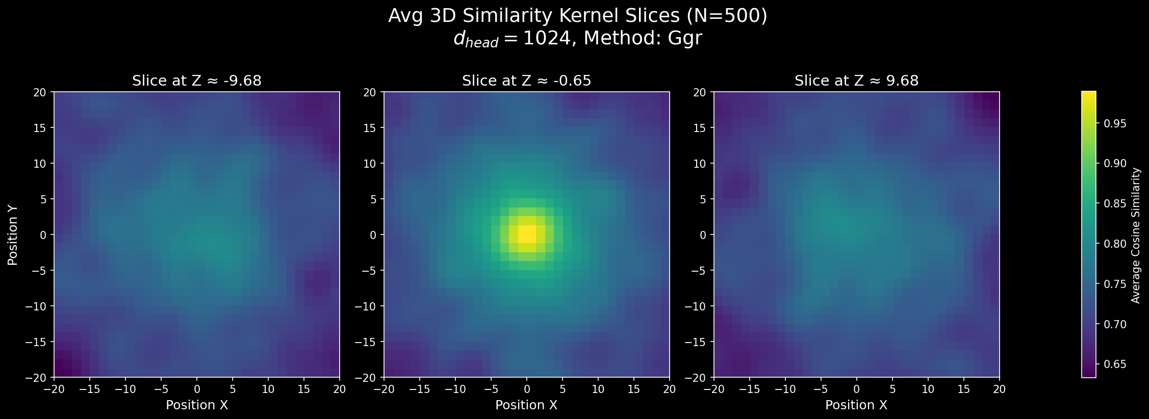
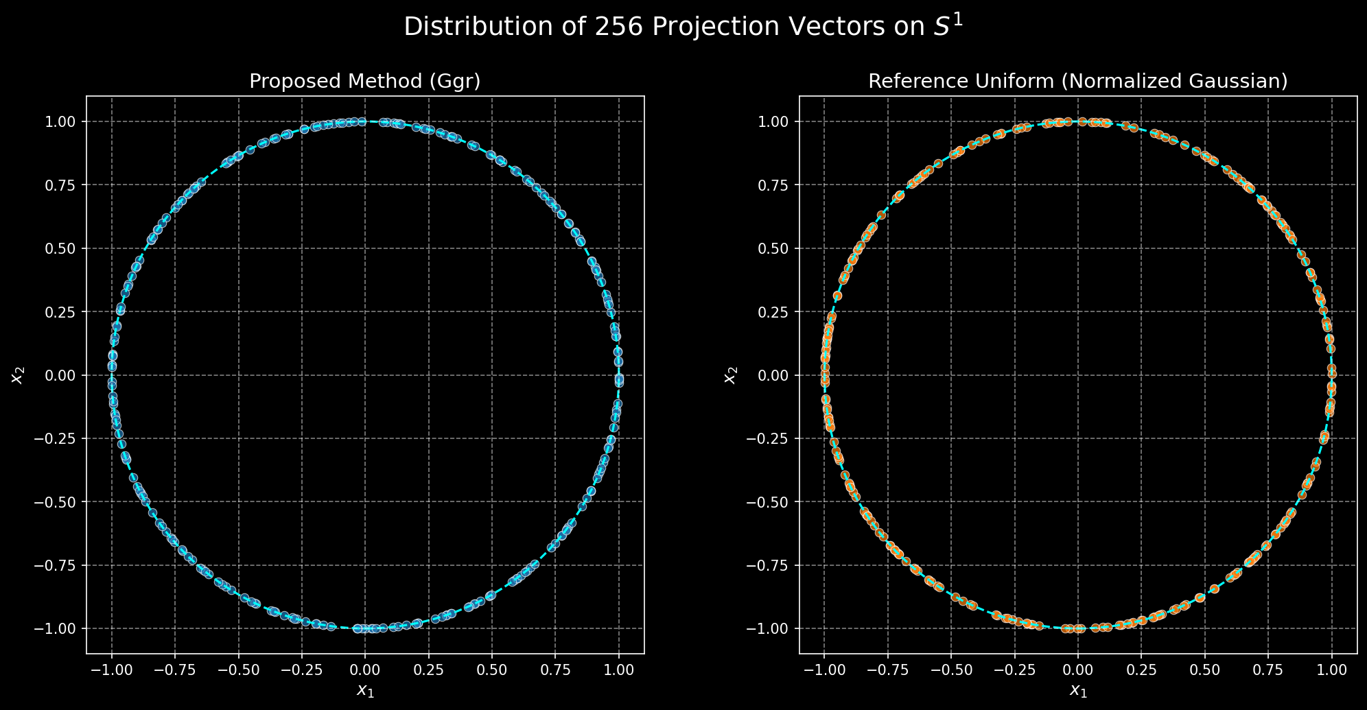
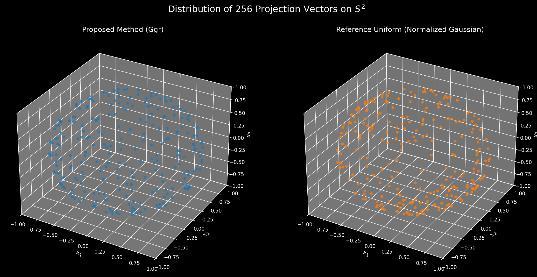
The challenge in extending RoPE to N dimensions (ND-RoPE) is choosing the projection vectors that map the $N$-dimensional position to a set of rotation angles. A good set of these vectors should have two key properties: uniformity and decorrelation. Uniformity means the vectors are spread out well (e.g., on the sphere $S^{n−1}$), ensuring all spatial directions are treated uniformly (at least without too much distortion needed from the dot product). Decorrelation (or incoherence) means the vectors are chosen such that the rotation angles for different feature pairs don’t have simple, repeating relationships, which would introduce unwanted structural dependencies. The following proposals attempt to solve for these properties.

There is a great blog post on 2D RoPE by Jerry Xiong here which shows how to pick such vectors for 2D RoPE that seems to beat other approaches to 2D RoPE (axial, random and learned).

The ND RoPE case is a bit contentious. Kevin Yin in his blog post says that incoherence matters more than uniformity. Upon further discussion it seems both incoherence and uniformity matter (uniformity in the sense of having terms expressible by a basis without too much distortion - small displacements should give somewhat decent coverage). Jerry’s random ND RoPE proposal technically works to at least give a good starting point for both incoherence and uniformity, since it feels like it should be true that the set of constant-sized sequences of linearly independent real numbers over $\mathbb{Q}$ that are also on $S^{n-1}$ are dense in the constant-sized sequences of points picked from $S^{n-1}$ itself. But we would in general like to have something more deterministic.

So as Kevin notes in his post, the structure of the golden ratio solution ignores the fact that the frequencies are exponential and not constant. We will similarly ignore this structure since it makes things quite hard otherwise. In a sense, you can think of our solutions as a limiting case when all the frequencies are rational.

The first solution I had for this while discussing this problem a month or so ago was related to square roots of square-free numbers (I forget what that construction exactly was), and though they provide good incoherence, it recently had some debate on whether it works or not.

So the second solution I had was to try and use these same things for constructing a uniform distribution inside a unit cube (noting by Weyl’s theorem that the fractional parts of integer multiples of irrational square roots are dense in $[0, 1]$) - pick $2 \{a_{ij} \sqrt{n_{in + j}}\} - 1$ where $n_k$ is the $k$-th square free positive integer. However, most of the mass is concentrated near the corners of the cube, which might do bad things to uniformity (as $N$ becomes large, it might concentrate things near the corners), and also interferes with the magnitude of the frequencies (if not normalized, but the previous issue holds in that case too). This works for $N = 1$ pretty well, however.

The third solution I had for $N > 1$ dimensions (using continued fractions), which seems to work, is as follows:

We want to sample points from Gaussians as closely as possible (we will then normalize them to lie on $S^{n-1}$, and since they’re independent, this will be close to a uniformly random choice on $S^{n-1}$). To do this, sample a pseudo-random number from $(0, 1)$ (preferably a low discrepancy method for all $n$ dimensions at once, like Sobol sequences or n-dimensional generalized golden ratio Weyl sequences - see code below for an implementation), apply the inverse CDF of the Gaussian to get a $N(0, 1)$ sample, take its fractional part, and then find the $a_{ij}’$ that gives $\{a_{ij}’ \sqrt{p_{in + j}}\}$ within an $\varepsilon$ radius of that value (where $p_k$ is the $k$-th prime, not square free numbers this time). Then we add the integer part of that sample to this value, resulting in a number of the form $a_{ij} \sqrt{p_{in + j}} + b_{ij}$. Taking $n$ of these samples, we get a sample pretty close to a Gaussian sample (in the limit as $\varepsilon$ goes to $0$). Normalizing this still preserves incoherence (note that this is why we use primes and not square-free numbers this time), and gives us a close to uniformly random point on $S^{n-1}$.

How do you do this efficiently? The answer is using continued fraction convergents. Note that the approximation error $|A_m - B_m \sqrt{p}|$ for each convergent drops exponentially, so to get an error of around $\varepsilon / 2$, we would need of the order of $\log \frac{1}{\epsilon}$ iterations. Then we can skip directly to the required multiple $a_{ij}$ of $B_m$ (by dividing and rounding) in a single step. This completes the solution.

Kevin also notes that it’s possible to build up a sequence of projections in a greedy fashion: adding a projection, then doing gradient descent to minimize the objective, so any scheme would have to be better than that. Or doing gradient descent starting from an initial set of points also works.

Here are some visualizations:

Some visualization code

Code written by Gemini 2.5 Pro, prompting and code fixes my own.

"""
Combined script to generate and visualize N-dimensional RoPE projections and similarity kernels.

This script unifies four methods for sampling points for projection generation and provides
a command-line interface to control the functionality.

Functionalities (Commands):
  - proj_viz: Visualize the distribution of projection vectors on a 2D or 3D sphere.
  - sim_2d:   Generate and visualize a 2D similarity kernel heatmap.
  - sim_3d:   Generate and visualize slices of a 3D similarity kernel.

Sampling Methods (`--sampling-method`):
  - ggr:      Uses a generalized golden ratio for low discrepancy.
  - sobol:    Uses a Sobol quasi-random sequence for sampling. (Requires scipy)
  - weyl:     Uses a Weyl sequence (also known as Kronecker sequence).
  - uniform:  Uses a standard pseudo-random uniform distribution.

Example Usage:

1. Visualize 256 2D projection vectors using the 'sobol' method:
   python rope_visualization.py proj_viz --n-dims 2 --num-vectors 256 --sampling-method sobol

2. Generate a 2D similarity kernel with d_head=512 using the 'weyl' method:
   python rope_visualization.py sim_2d --d-head 512 --sampling-method weyl

3. Generate 3D similarity kernel slices with 500 samples using the 'ggr' method:
   python rope_visualization.py sim_3d --num-samples 500 --sampling-method ggr
"""
import math
import numpy as np
from scipy.stats import norm
from scipy.stats.qmc import Sobol
from pathlib import Path
import matplotlib.pyplot as plt
import concurrent.futures
import os
from tqdm import tqdm
import argparse
from typing import List, Tuple

def get_primes(count: int) -> List[int]:
    if count <= 0:
        return []
    if count < 6:
        limit_est = 15
    else:
        log_c = math.log(count)
        limit_est = int(count * (log_c + math.log(log_c))) + 10

    primes_list = []
    while len(primes_list) < count:
        is_prime = [True] * limit_est
        if limit_est > 0: is_prime[0] = False
        if limit_est > 1: is_prime[1] = False
        for p in range(2, int(math.sqrt(limit_est)) + 1):
            if is_prime[p]:
                for multiple in range(p * p, limit_est, p):
                    is_prime[multiple] = False
        primes_list = [i for i, prime in enumerate(is_prime) if prime]
        if len(primes_list) < count:
            limit_est *= 2
    return primes_list[:count]

def get_continued_fraction_convergents(
    alpha: float, n_terms: int, error: float
) -> Tuple[List[int], List[int]]:
    p = [0, 1]
    q = [1, 0]
    alpha_original = alpha
    for _ in range(n_terms):
        if alpha == math.floor(alpha):
            break
        a = math.floor(alpha)
        p.append(a * p[-1] + p[-2])
        q.append(a * q[-1] + q[-2])
        if abs(q[-1] * alpha_original - p[-1]) < error:
            break
        alpha = 1.0 / (alpha - a)
    return p[2:], q[2:]

def generate_nd_rope_projections(
    d_head: int,
    n_dims: int,
    sampling_method: str,
    cf_terms: int = 20,
    error: float = 1e-4,
) -> np.ndarray:
    if d_head % 2 != 0:
        raise ValueError("d_head must be an even number.")
    num_projections = d_head // 2
    num_total_samples = num_projections * n_dims

    print(f"Generating samples using '{sampling_method}' method...")
    if sampling_method == 'sobol':
        sobol_gen = Sobol(d=n_dims, scramble=True)
        samples = sobol_gen.random(n=num_projections).flatten()
    elif sampling_method == 'weyl':
        primes_for_weyl = get_primes(n_dims)
        generators = np.sqrt(np.array(primes_for_weyl))
        generators = generators - np.floor(generators)
        arange_col = np.arange(1, num_projections + 1).reshape(-1, 1)
        weyl_samples = arange_col * generators
        samples = (weyl_samples - np.floor(weyl_samples)).flatten()
    elif sampling_method == 'uniform':
        samples = np.random.uniform(0, 1, size=num_total_samples)
    elif sampling_method == 'ggr':
        l, r = 1, 2
        for _ in range(100):
            m = (l + r) / 2
            if m ** (n_dims + 1) < m + 1:
                l = m
            else:
                r = m
        generators = np.exp(np.arange(1, n_dims + 1) * np.log(1 / l))
        generators = generators - np.floor(generators)
        arange_col = np.arange(1, num_projections + 1).reshape(-1, 1)
        ggr_samples = arange_col * generators
        samples = (ggr_samples - np.floor(ggr_samples)).flatten()
    else:
        raise ValueError(f"Unknown sampling method: {sampling_method}")

    print(f"Generating {num_projections} projection vectors of {n_dims} dimensions...")
    print(f"Needing {num_total_samples} prime numbers for approximation...")
    primes = get_primes(num_total_samples)
    print("Primes generated.")

    projection_vectors = np.zeros((num_projections, n_dims))
    prime_idx, sample_idx = 0, 0

    for i in tqdm(range(num_projections), desc=f"Generating {n_dims}D Projections"):
        vec = np.zeros(n_dims)
        for j in range(n_dims):
            prime = primes[prime_idx]
            alpha = math.sqrt(prime)
            prime_idx += 1

            u = samples[sample_idx]
            sample_idx += 1

            y_target = norm.ppf(u)
            y_int = math.floor(y_target)
            y_frac = y_target - y_int

            p_conv, q_conv = get_continued_fraction_convergents(alpha, cf_terms, error / 4)
            if not p_conv:
                vec[j] = y_int
                continue

            pn, qn = p_conv[-1], q_conv[-1]
            delta = qn * alpha - pn

            j_mult = round(y_frac / delta) if abs(delta) > 1e-18 else 0
            a = j_mult * qn
            k = j_mult * pn
            vec[j] = abs(a * alpha - k) + y_int

        norm_val = np.linalg.norm(vec)
        projection_vectors[i] = vec / norm_val

    print("Projection vectors generated successfully.")
    return projection_vectors

def _calculate_rope_similarity(q, k, positions, projections, base_thetas):
    d_head = q.shape[0]
    q_norm = q / np.linalg.norm(q)
    k_norm = k / np.linalg.norm(k)
    q_pairs = q_norm.reshape(d_head // 2, 2)
    k_pairs = k_norm.reshape(d_head // 2, 2)
    angles = (positions @ projections.T) * base_thetas
    cos_a, sin_a = np.cos(angles), np.sin(angles)
    term1 = np.sum(q_pairs * k_pairs, axis=1)
    term2 = q_pairs[:, 0] * k_pairs[:, 1] - q_pairs[:, 1] * k_pairs[:, 0]
    dot_products = (term1 * cos_a + term2 * sin_a).sum(axis=1)
    return dot_products

def _calculate_single_sample_similarity(d_head, positions, projections, base_thetas):
    q = np.random.randn(d_head)
    return _calculate_rope_similarity(q, q, positions, projections, base_thetas)

def visualize_projections(
    n_dims: int,
    num_vectors: int,
    sampling_method: str,
    save_path: str
):
    if n_dims not in [2, 3]:
        raise ValueError("Visualization is only supported for n_dims=2 or 3.")

    our_vectors = generate_nd_rope_projections(
        d_head=num_vectors * 2, n_dims=n_dims, sampling_method=sampling_method
    )
    ref_vectors = np.random.randn(num_vectors, n_dims)
    ref_vectors /= np.linalg.norm(ref_vectors, axis=1, keepdims=True)

    plt.style.use('dark_background')
    fig_title = f"Distribution of {num_vectors} Projection Vectors on $S^{{{n_dims-1}}}$"

    if n_dims == 2:
        fig, (ax1, ax2) = plt.subplots(1, 2, figsize=(14, 7))
        fig.suptitle(fig_title, fontsize=18)
        titles = [f"Proposed Method ({sampling_method.capitalize()})", "Reference Uniform (Normalized Gaussian)"]
        for ax, data, title, color in zip([ax1, ax2], [our_vectors, ref_vectors], titles, ['#1f77b4', '#ff7f0e']):
            ax.scatter(data[:, 0], data[:, 1], alpha=0.7, edgecolors='w', linewidth=0.5, c=color)
            circle = plt.Circle((0, 0), 1, color='cyan', fill=False, linestyle='--', linewidth=1.5)
            ax.add_artist(circle)
            ax.set_title(title, fontsize=14)
            ax.set_xlabel("$x_1$", fontsize=12)
            ax.set_ylabel("$x_2$", fontsize=12)
            ax.set_aspect('equal', adjustable='box')
            ax.set_xlim(-1.1, 1.1); ax.set_ylim(-1.1, 1.1)
            ax.grid(True, linestyle='--', alpha=0.5)
    elif n_dims == 3:
        fig = plt.figure(figsize=(16, 8))
        fig.suptitle(fig_title, fontsize=18)
        ax1 = fig.add_subplot(1, 2, 1, projection='3d')
        ax1.scatter(our_vectors[:, 0], our_vectors[:, 1], our_vectors[:, 2], alpha=0.7, c='#1f77b4')
        ax1.set_title(f"Proposed Method ({sampling_method.capitalize()})", fontsize=14)
        ax2 = fig.add_subplot(1, 2, 2, projection='3d')
        ax2.scatter(ref_vectors[:, 0], ref_vectors[:, 1], ref_vectors[:, 2], alpha=0.7, c='#ff7f0e')
        ax2.set_title("Reference Uniform (Normalized Gaussian)", fontsize=14)
        for ax in [ax1, ax2]:
            ax.set_xlabel("$x_1$", fontsize=12); ax.set_ylabel("$x_2$", fontsize=12); ax.set_zlabel("$x_3$", fontsize=12)
            ax.set_xlim(-1, 1); ax.set_ylim(-1, 1); ax.set_zlim(-1, 1)

    plt.tight_layout(rect=[0, 0.03, 1, 0.95])
    plt.savefig(save_path, dpi=150, bbox_inches='tight')
    plt.close(fig)
    print(f"\nProjection visualization saved to '{save_path}'")

def visualize_similarity_kernel_2d(
    d_head: int, grid_size: int, num_samples: int, sampling_method: str, save_path: str
):
    cores = os.cpu_count()
    print(f"\nGenerating 2D similarity kernel (avg over {num_samples} samples, {cores} cores)...")
    projections = generate_nd_rope_projections(d_head=d_head, n_dims=2, sampling_method=sampling_method)
    base_thetas = 1.0 / (10000 ** (np.arange(0, d_head, 2, dtype=np.float32) / d_head))
    plot_range = 20.0
    r = np.linspace(-plot_range, plot_range, grid_size)
    i, j = np.meshgrid(r, r)
    positions = np.vstack([i.ravel(), j.ravel()]).T
    accumulated_similarity = np.zeros(positions.shape[0])

    with concurrent.futures.ProcessPoolExecutor() as executor:
        futures = [executor.submit(_calculate_single_sample_similarity, d_head, positions, projections, base_thetas) for _ in range(num_samples)]
        for f in tqdm(concurrent.futures.as_completed(futures), total=num_samples, desc="Processing samples"):
            accumulated_similarity += f.result()

    similarity_map = (accumulated_similarity / num_samples).reshape(i.shape)
    plt.style.use('dark_background')
    fig, ax = plt.subplots(figsize=(9, 7))
    im = ax.imshow(similarity_map, origin='lower', extent=[-plot_range, plot_range, -plot_range, plot_range], cmap='viridis')
    cbar = fig.colorbar(im, ax=ax, label="Average Cosine Similarity", pad=0.04)
    cbar.ax.yaxis.label.set_color('white'); cbar.ax.tick_params(axis='y', colors='white')
    ax.set_title(f"Average Similarity Kernel (2D, N={num_samples})\n$d_{{head}}={d_head}$, Method: {sampling_method.capitalize()}", fontsize=16, pad=12)
    ax.set_xlabel("Position X", fontsize=12); ax.set_ylabel("Position Y", fontsize=12)
    ax.grid(False)
    plt.savefig(save_path, dpi=150, bbox_inches='tight')
    plt.close(fig)
    print(f"2D similarity kernel saved to '{save_path}'")

def visualize_similarity_kernel_3d_slices(
    d_head: int, grid_size: int, num_samples: int, slice_coords: list[float], sampling_method: str, save_path: str
):
    cores = os.cpu_count()
    print(f"\nGenerating 3D similarity kernel slices (avg over {num_samples} samples, {cores} cores)...")
    projections = generate_nd_rope_projections(d_head=d_head, n_dims=3, sampling_method=sampling_method)
    base_thetas = 1.0 / (10000 ** (np.arange(0, d_head, 2, dtype=np.float32) / d_head))
    plot_range = 20.0
    r = np.linspace(-plot_range, plot_range, grid_size)
    i, j, k_grid = np.meshgrid(r, r, r, indexing='ij')
    positions = np.vstack([i.ravel(), j.ravel(), k_grid.ravel()]).T
    accumulated_similarity = np.zeros(positions.shape[0])

    with concurrent.futures.ProcessPoolExecutor() as executor:
        futures = [executor.submit(_calculate_single_sample_similarity, d_head, positions, projections, base_thetas) for _ in range(num_samples)]
        for f in tqdm(concurrent.futures.as_completed(futures), total=num_samples, desc="Processing samples"):
            accumulated_similarity += f.result()

    similarity_volume = (accumulated_similarity / num_samples).reshape(i.shape)
    vmin, vmax = similarity_volume.min(), similarity_volume.max()
    plt.style.use('dark_background')
    num_slices = len(slice_coords)
    fig, axes = plt.subplots(1, num_slices, figsize=(5 * num_slices, 5.5), constrained_layout=True)
    if num_slices == 1: axes = [axes]
    fig.suptitle(f"Avg 3D Similarity Kernel Slices (N={num_samples})\n$d_{{head}}={d_head}$, Method: {sampling_method.capitalize()}", fontsize=18)

    for ax, z_coord in zip(axes, slice_coords):
        slice_idx = np.argmin(np.abs(r - z_coord))
        im = ax.imshow(similarity_volume[:, :, slice_idx].T, origin='lower', extent=[-plot_range, plot_range, -plot_range, plot_range], cmap='viridis', vmin=vmin, vmax=vmax)
        ax.set_title(f"Slice at Z ≈ {r[slice_idx]:.2f}", fontsize=14)
        ax.set_xlabel("Position X", fontsize=12)
        ax.grid(False)
    axes[0].set_ylabel("Position Y", fontsize=12)
    cbar = fig.colorbar(im, ax=axes, label="Average Cosine Similarity", shrink=0.8, pad=0.08)
    cbar.ax.yaxis.label.set_color('white'); cbar.ax.tick_params(axis='y', colors='white')
    plt.savefig(save_path, dpi=150, bbox_inches='tight')
    plt.close(fig)
    print(f"3D similarity slices saved to '{save_path}'")

def main():
    parser = argparse.ArgumentParser(
        description="Generate and visualize N-dimensional RoPE projections and similarity kernels.",
        formatter_class=argparse.RawTextHelpFormatter,
        epilog="""\
Example Usage:
  # Visualize 2D projections with the 'sobol' method
  python %(prog)s proj_viz --n-dims 2 --num-vectors 256 --sampling-method sobol

  # Generate 2D similarity kernel with the 'weyl' method
  python %(prog)s sim_2d --d-head 512 --sampling-method weyl

  # Generate 3D similarity slices with the 'uniform' method
  python %(prog)s sim_3d --d-head 512 --num-samples 500 --sampling-method uniform
"""
    )
    subparsers = parser.add_subparsers(dest='command', required=True, help='Select the task to run')

    sampling_choices = ['ggr', 'sobol', 'weyl', 'uniform']

    parser_proj = subparsers.add_parser('proj_viz', help='Visualize projection vector distribution on a sphere.')
    parser_proj.add_argument('--n-dims', type=int, choices=[2, 3], required=True, help='Number of dimensions for the projections (2 or 3).')
    parser_proj.add_argument('--num-vectors', type=int, required=True, help='Number of projection vectors to generate.')
    parser_proj.add_argument('--sampling-method', type=str, choices=sampling_choices, default='sobol', help='Method for sampling points in [0, 1).')
    parser_proj.add_argument('--save-path', type=str, default=None, help='Path to save the plot. Defaults to "rope_viz_[n_dims]d_[method].png".')

    parser_sim2d = subparsers.add_parser('sim_2d', help='Visualize a 2D similarity kernel.')
    parser_sim2d.add_argument('--d-head', type=int, default=1024, help='The dimension of the head vector.')
    parser_sim2d.add_argument('--grid-size', type=int, default=64, help='The number of points along each axis of the position grid.')
    parser_sim2d.add_argument('--num-samples', type=int, default=500, help='Number of random query vectors to average over.')
    parser_sim2d.add_argument('--sampling-method', type=str, choices=sampling_choices, default='sobol', help='Method for sampling points in [0, 1).')
    parser_sim2d.add_argument('--save-path', type=str, default='rope_similarity_2d_avg.png', help='Path to save the plot.')

    parser_sim3d = subparsers.add_parser('sim_3d', help='Visualize slices of a 3D similarity kernel.')
    parser_sim3d.add_argument('--d-head', type=int, default=1024, help='The dimension of the head vector.')
    parser_sim3d.add_argument('--grid-size', type=int, default=32, help='The number of points along each axis of the position grid.')
    parser_sim3d.add_argument('--num-samples', type=int, default=500, help='Number of random query vectors to average over.')
    parser_sim3d.add_argument('--slice-coords', type=float, nargs='+', default=[-10.0, 0.0, 10.0], help='A list of Z-coordinates for the slices.')
    parser_sim3d.add_argument('--sampling-method', type=str, choices=sampling_choices, default='sobol', help='Method for sampling points in [0, 1).')
    parser_sim3d.add_argument('--save-path', type=str, default='rope_similarity_3d_slices_avg.png', help='Path to save the plot.')

    args = parser.parse_args()

    if args.command == 'proj_viz':
        save_path = args.save_path or f"rope_viz_{args.n_dims}d_{args.sampling_method}.png"
        visualize_projections(
            n_dims=args.n_dims, num_vectors=args.num_vectors,
            sampling_method=args.sampling_method, save_path=save_path
        )
    elif args.command == 'sim_2d':
        visualize_similarity_kernel_2d(
            d_head=args.d_head, grid_size=args.grid_size, num_samples=args.num_samples,
            sampling_method=args.sampling_method, save_path=args.save_path
        )
    elif args.command == 'sim_3d':
        visualize_similarity_kernel_3d_slices(
            d_head=args.d_head, grid_size=args.grid_size, num_samples=args.num_samples,
            slice_coords=args.slice_coords, sampling_method=args.sampling_method,
            save_path=args.save_path
        )

if __name__ == '__main__':
    if os.name == 'posix':
        import multiprocessing
        multiprocessing.set_start_method('fork')
    main()

Introduction#

The Problem#

The Solution#

The other proof#

Coming up with these vectors#

Introduction

The Problem

The Solution

The other proof

Coming up with these vectors